 2015, Vol. 58


在位场数据的处理方法技术中,垂向导数在划分区域场和局部异常、分离叠加异常、边界识别(Verduzco et al., 2004; 王万银等,2010; 马国庆等,2012; 王彦国等,2013)、异常反演(Marson and Klingele, 1993; Cooper,2004; Doo et al., 2007; 张恒磊等,2012; 马国庆等,2014b)等方面都有重要作用.通常认为,垂向导数的换算是不稳定的,且阶数越高,换算越不稳定.位场垂向导数换算的方法很多,但大致可以分为两类:一是空间域法;二是波数域法.空间域法包括最初的量板法和泰勒级数近似法(曾华霖,2005; 管志宁,2005)、边界单元法和有限元法(徐世浙, 1984a,1984b)、样条函数法(王硕儒等,1987; 汪炳柱,1996; 姚长利等,1997; Wang et al., 2008)等. 波数域法包括原始的常规算子法、 维纳滤波法(Clarke,1969; Gupta and Ramani, 1982)、 补偿圆滑滤波法(侯重初,1981)、正则化方法(Pašteka et al., 2009)等.针对Fourier变换复数运算的复杂性,两种实数域内的变换:余弦变换(张凤旭等, 2006,2007)和Hartley变换(Sundararajan and Brahmam, 1998; 魏雅利和骆遥,2011)被引入到垂向导数的换算,但这两种变换方法仅仅是计算量的减少,垂向导数换算的精度并没有提高(刘东甲等,2012; 马国庆等,2014a).为了避免高阶垂向导数换算的不稳定性,也有文献采用分数阶垂向导数(Gunn et al., 1997; Cooper and Cowan, 2003,2004; Cowan and Cooper, 2005)来平衡特征增强效果和噪声放大效应.
Fedi和Florio(2001)基于位场及其各阶垂向导数都满足Laplace方程的基本原理,提出空间域和频率域相结合的换算各阶垂向导数的ISVD(integrated second vertical derivative)算法.该方法首先在频率域中对位场进行垂向积分得到位场的标量位,然后在空间域采用有限差分法分别求原位场及其标量位的水平二阶导数,并由Laplace方程计算各自的垂向二阶导数,进而分别得到位场的垂向一阶和二阶导数,最后以此类推,得到位场的各阶垂向导数.目前,ISVD算法已经成为稳定求解位场各阶垂向导数的主流方法,在位场数据处理的许多领域中得到广泛 应用(Fedi and Florio, 2002; Trompat,2003; Cooper,2004; 翟国君等,2011; Paoletti et al., 2013; 卞光浪等,2014).
本文提出一种新的正则化方法用于位场各阶垂向导数的换算.新正则化方法从位场径向平均功率谱(Spector and Grant, 1970)的物理特性出发,定义一个截止波数来划分位场功率谱,并由此构建更优的正则低通滤波函数;然后,令定义的截止波数等于正则低通滤波函数的截止波数来求解正则参数.新正则化方法具有物理意义明确、计算简单的优点.通过单个和组合理论重力模型及实测航磁数据对基于ISVD算法和新正则化方法的位场各阶垂向导数换算和泰勒级数法向下延拓进行了对比实验,结果表明,新正则化方法优势明显.
2 位场垂向导数换算的正则化方法及其改进位场T(x,y)与其各阶垂向导数Di(x,y)(i代表阶数)在波数域的关系式为

 为径向波数;(2πωr)i为各阶垂向导数算子.由于(2πωr)i的噪声放大特性,导致换算结果Di(ωx,ωy)的不稳定性,且导数的阶数越高,换算结果越不稳定.
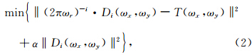
针对求解形如(1)式的不稳定问题,Tikhonov正则化是一种广泛应用的方法,它指的是求解一个极小化的正则化泛函(王彦飞,2007; Pašteka et al., 2009)
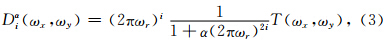
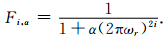 正是由于正则低通滤波函数抑制了T(ωx,ωy)中的噪声干扰,才使Tikhonov正则垂向导数换算的结果趋于稳定.
定性地讲,如果我们简单地假设将实际观测位场T(ωx,ωy)看成是深源长波长位场Td(ωx,ωy)与浅源短波长位场Ts(ωx,ωy)的叠加

正则化方法实现的关键在于最优正则参数的选 取,其关系到正则化方法的计算精度和计算时间.常用的正则参数选取方法有L-曲线法、GCV(generalized cross validation)法、拟最优准则(或称C-范数法(Pašteka et al., 2009; Zhang et al., 2013))、偏差准则等(王彦飞,2007).这些方法的共同点是:首先,设定一个取值范围较广的等比级数序列作为正则参数的离散值,当然,为了提高计算精度,离散值的个数越多越好;其次,计算每个离散正则参数对应的正则化结果,然后,根据一定的准则来选择最优的正则参数.比如,L-曲线法的拐点或最大曲率、GCV曲线的最小值、C-范数曲线的局部最小值、满足偏差准则方程的正则参数等.从以上的描述可知,要得到精确的最优正则参数,上述所有正则参数选取方法都存在计算量偏大的问题.本文拟在分析位场径向平均功率谱、定义其截止波数的基础上,得出正则参数和截止波数的关系,将正则参数的选取问题转换为确定径向功率谱的截止波数,以此来避免常规正则参数计算量偏大的问题.
Spector和Grant(1970)提出径向平均功率谱的概念,并被广泛应用于位场数据处理(Maus and Dimri, 1995; Ravat et al., 2007; 郭良辉等,2012;Guo et al., 2013).径向谱的定义如下:设位场数据的功率谱为P(ωx,ωy),其在径向方向φ上的取值为P′(ωr,φ),则

一个假想的径向平均功率谱如图 1所示.从图 1可知,如果假设观测噪声为白噪声,则与位场信号不相关的白噪声的功率谱应该为常数,即对应于图 1中的水平部分.如此,对于位场的径向平均功率谱,存在一个截止径向波数ω′ c将位场信号谱和噪声谱大致分开.
 | 图 1 径向平均功率谱示意图Fig. 1 The schematic diagram for the radially averaged power spectrum |
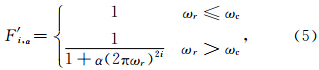
在第2节中,我们正好需要确定一个截止波数ωc来定义改进的正则低通滤波函数F′ i,α.由此,可以简单地定义ωc为通过径向平均功率谱确定的截止径向波数ω′ c.同时,如果设定截止波数ωc为正则低通滤波函数Fi,α的截止波数(定义为Fi,α的值降为0.5时的ωr值),则可以简单地得到正则参数α和截止波数ωc的关系为

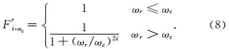
当然,也存在截止波数ω′ c不易确定的情况.主要有以下两种情况:(1)重磁位场实际数据在进行诸如求导、化极、向下延拓等不稳定换算时,通常先进行低通滤波预处理以减少高频噪声对换算结果的影响(曾华霖,2005; 管志宁,2005).低通滤波后的重磁位场数据,由于高频噪声被滤除,功率谱曲线转折点不明显,导致截止波数不易确定;(2)当重磁位场实际数据高频分量比较丰富且噪声干扰少时,重磁位场实际数据高频分量的径向功率谱容易淹没高频噪声的径向功率谱,导致截止波数不易确定.针对以上两种情况,在应用本文方法进行垂向导数换算时,不需对重磁位场实际数据进行低通滤波预处理,且原始数据噪声干扰越大越易确定截止波数.同时,对于噪声干扰少的高精度重磁位场数据,可适当添加白噪声以利于确定截止波数.由正则低通滤波函数F′ i,ωc的滤波特性,添加的白噪声将被滤除而对换算结果不会产生影响.
4 理论模型实验 4.1 单个球体模型球心位于坐标原点,埋深为2.5 km,半径为2 km,点、线距同为0.1 km,与围岩密度差为1 g·cm-3的球体所引起的重力异常如图 2a所示.为模拟实际情况,给原始重力异常值增加零均值、方差为0.02的高斯白噪声(信噪比为29.84 dB),其结果如图 2b所示.计算含噪重力异常的径向平均功率谱,如图 2c所示(虚线为径向谱中拟合得到的线性部分),则通过功率谱形状分析,可将功率谱分为0~0.00059和0.00059~0.005两段.将前段视为信号部分,后一段近似视为噪声部分,如此,则可以确定功率谱的截止波数为ωc=0.00059.根据第3节末尾的分析,在实际资料处理中,径向功率谱曲线的转折点可能不明显而导致截止波数的确定存在偏差.为了研究截止波数对各阶垂向导数换算的影响,另取两个截止波数分别为ωc1=0.0003和ωc2=0.0009进行正则各阶垂向导数换算实验.
 | 图 2 理论单个球体模型重力数据前三阶垂向导数效果对比 (a)重力数据等值线图;(b)含噪重力数据等值线图及其(c)径向对数功率谱; 换算结果在主剖面的对比值:(d)一阶垂向导数,(e)二阶垂向导数,(f)三阶垂向导数.Fig. 2 Effects comparison of the first three vertical derivatives based on the model gravity data for the single sphere (a)Contours of gravity data;(b)Contours of gravity data with noise and (c)its radially averaged power spectrum; The conversion results in the main profile for(d)the first vertical derivative,(e)the second vertical derivative, and (f)the three vertical derivative. |
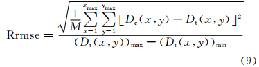
在图 2b的基础上,分别采用ISVD算法和本文提出的新正则化方法计算模型前三阶垂向导数.由于ISVD算法在采用有限差分法计算位场及其梯度的水平导数时会放大噪声,因此,在计算二阶及三阶垂向导数前,我们采用5×5的平滑(均值)滤波器模板对位场及其梯度进行了消噪处理.两种方法的计算结果和理论值在主剖面的对比如图 2d、2e、2f所示(本文方法仅显示截止波数为ωc=0.00059时的换算结果).同时,各阶垂向导数的计算值Dc(x,y)和理论值Dt(x,y)通过相对均方根误差Rrmse(Relative root mean square error)(Wang et al., 2008)
| 表 1 ISVD算法和本文方法前三阶垂向导数换算误差对比Table 1 The conversion errors of the first three vertical derivatives for ISVD and the proposed method |
理论组合球体模型由两个不同深度层、不同大小的7个球体组合而成,图 3a显示了它们在直角坐标系(设z坐标向下为正)中的位置.各球体的具体 参数见表 2.设点、线数同为512,点、线距都为50 m.
 | 图 3 理论组合球体模型重力数据垂向二阶导数和向下延拓效果对比 (a)球体位置坐标系;(b)h=0 m高度含噪重力数据等值线图及其(c)径向对数功率谱;(d)理论二阶垂向导数等值线图; 两种方法的垂向二阶导数换算结果:(e)ISVD算法;(f)本文方法;(g)h=1000 m高度重力数据等值线图;(h)ISVD算法采用前三阶垂向导数进行泰勒级数法向下延拓的结果; 本文方法采用(i)前三阶、(j)前五阶、(k)前七阶、(l)前九阶垂向导数进行泰勒级数法向下延拓的结果.Fig. 3 Effects comparison of the second vertical derivative and downward continuation based on the model gravity data for the group sphere (a)Location of spheres coordinates system;(b)Contours of gravity data with noise at h=0 m and (c)its radially averaged power spectrum;(d)Contours of the exact second vertical derivative data; the conversion second vertical derivative results for(e)the ISVD method and (f)the proposed method;(g)Contours of gravity data at h=1000 m;(h)The downward continuation results of the Taylor series method based on the calculation of the first three vertical derivatives using the ISVD algorithm; The downward continuation results of the Taylor series method based on the calculation of(i)the first three vertical derivatives,(j)the first five vertical derivatives,(k)the first seven vertical derivatives and (l)the first nine vertical derivatives using the proposed method. |
| 表 2 仿真球体所用参数Table 2 Parameters of simulation spheres |
实验中,以h=0 m高度的重力异常数据为观测数据,并加入零均值、方差为0.0005 mGal的高斯白噪声(信噪比为36.06 dB)来模拟实际情况,其结果如图 3b所示.首先,计算图 3b中含噪重力异常数 据的径向平均功率谱,如图 3c所示(虚线为径向谱中拟合得到的线性部分).通过功率谱形状分析,显然可将功率谱分为三段,将前两段视为信号部分,后一段近似视为噪声部分,如此,则可以确定功率谱的截止波数为ωc=0.00086.模型二阶垂向导数的理论值如图 3d所示.分别采用ISVD算法和本文方法在图 3b所示含噪重力异常数据的基础上求二阶导数,其结果分别如图 3e(Rrmse=5.74%;Re= 44.65%)和图 3f(Rrmse=0.75%;Re=3.39%)所示.
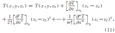
为了更加全面地对比各阶垂向导数的换算精度,在ISVD算法和本文所提方法求得各阶垂向导数的基础上,利用泰勒级数法进行位场的向下延拓对比实验.位场泰勒级数法向下延拓的原理如下(Evjen,1936; Fedi and Florio, 2002; 卞光浪等,2014)
由图 3e和图 3f、图 3h和图 3i—3l的对比可知:(1)由于采用空间域有限差分法计算位场水平导数存在误差,ISVD算法在计算各阶垂向导数时同样存在误差,且误差具有累积效应,阶数越高,误差越大,最终导致基于该方法的位场泰勒级数法向下延拓很不稳定.这也是该方法向下延拓的距离非常有限的原因(Fedi and Florio, 2002; Xu,2007; 卞光浪等,2014);(2)利用新正则化方法得到的各阶垂向导数结果进行泰勒级数法向下延拓可以取得大深度、高精度的向下延拓结果.
5 航磁实测数据下延实验航磁实测数据点距和线距均为100 m,如图 4a所示.将原始数据向上延拓1000 m(10倍点距)以构建另一个平面的数据(图 4b);同时,考虑到向上延拓具有的平滑效应,为模拟实际情况,本文在向上 延拓后得到的航磁数据中加入零均值、方差为5.75 nT 的高斯白噪声(信噪比为35.49 dB),加噪后航磁数据如图 4c所示.计算该含噪航磁数据的径向平均功率谱,结果如图 4d所示(虚线为径向谱中拟合得到的线性部分).通过径向谱形状分析,可以确定径向谱的截止波数为ωc=0.00082.
 | 图 4 实测航磁数据向下延拓效果对比 (a)原始航磁等值线图;(b)向上延拓10倍点距后等值线图;(c)向上延拓航磁异常加噪数据等值线图及其(d)径向对数功率谱;(e)ISVD算法采用前三阶垂向导数进行泰勒级数法向下延拓的结果; 本文方法采用(f)前三阶、(g)前五阶、(h)前七阶、(i)前九阶垂向导数进行泰勒级数法向下延拓的结果.Fig. 4 Effects comparison of downward continuation based on the real aeromagnetic data (a)Contours of the original aeromagnetic data;(b)Upward continuation 10 grid interval;(c)Contours of upward continuation aeromagnetic data with noise and (d)its radially averaged power spectrum;(e)The downward continuation results of the Taylor series method based on the calculation of the first three vertical derivatives using the ISVD algorithm; The downward continuation results of the Taylor series method based on the calculation of(f)the first three vertical derivatives,(g)the first five vertical derivatives,(h)the first seven vertical derivatives and (i)the first nine vertical derivatives using the proposed method. |
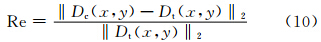
向下延拓实验为采用泰勒级数法(公式(11))将向上延拓后加噪的航磁数据(图 4c)向下延拓回原来的高度.同样,将向下延拓数据与原始航磁数据采用公式(9)和公式(10)(将各阶垂向导数值换成航磁数据)进行误差对比.ISVD算法采用前三阶垂向导 数进行位场向下延拓的结果如图 4e(Rrmse=2.13%; Re=11.46%)所示.本文方法采用前三阶、前五阶、前七阶、前九阶进行向下延拓的结果分别如图 4f(Rrmse=1.40%;Re=9.76%)、图 4g(Rrmse= 1.24%;Re=6.60%)、图 4h(Rrmse=1.32%;Re=6.20%)、图 4i(Rrmse=1.36%;Re=6.27%). 由图 4e—4i可见:(1)和理论模型一样,利用本文方法计算各阶垂向导数的结果进行泰勒级数法向下延拓可以获得比ISVD算法更加稳定、更加精确的结果;(2)利用本文方法计算各阶垂向导数的结果进行泰勒级数法向下延拓时,并不是阶数越多,结果越精确,原因是,每次波数域垂向导数的换算都引入了一定量的误差,采用的阶数越多,叠加起来后,误差也会达到一定的量.
6 结论(1)由于存在一次波数域积分运算和采用空间域有限差分法计算位场水平导数,ISVD算法在计算各阶垂向导数时,误差具有累积效应,偶数阶垂向导数累积了空间域水平导数计算的误差,奇数阶垂向导数换算累积了波数域积分运算误差(由吉布斯效应产生)和空间域水平导数计算所产生误差的双重误差,最终导致垂向导数换算的阶数越高,误差越大.要改变这种状况,ISVD需要高精度的水平导数求解方法.但是,空间域计算方法的精度一般都受网格间距的影响,且高精度的空间域方法总体比较复杂(Roy,2013).
(2)由于ISVD算法计算各阶垂向导数的精度有限,导致基于该方法的泰勒级数法向下延拓很不稳定,这也是原来的泰勒级数法向下延拓的距离非常有限的原因.
(3)本文提出的新正则化方法在计算各阶垂向导数时,虽然基于同一截止波数,但各个计算都是独立的,不存在误差的累积,因此,各阶垂向导数的计算误差都差不多,且计算各阶垂向导数的稳定性和精度明显优于ISVD法.
(4)在用本文方法获得高精度各阶垂向导数换算结果的基础上,泰勒级数法可以获得大深度、高精度的向下延拓结果.但值得注意的一点是,并不是泰勒级数近似的阶数越多,结果就越精确,原因是,每次波数域垂向导数的换算都引入了一定量的误差(由吉布斯效应和正则化过程产生),阶数越多,误差叠加得也越多,最终导致向下延拓的误差反而会增大.
| [1] | Bian G L, Zhai G J, Gao J Y, et al. 2014. Improved Taylor series approach for stable downward continuation of total strength of geomagnetic field. Acta Geodaetica et Cartographica Sinica (in Chinese), 43(1):30-36. |
| [2] | Clarke G K C. 1969. Optimum second-derivative and downward-continuation filters. Geophysics, 34(3):424-437. |
| [3] | Cooper G R J. 2004. Euler deconvolution applied to potential field gradients. Exploration Geophysics, 35(3):165-170. |
| [4] | Cooper G R J, Cowan D R. 2003. The application of fractional calculus to potential field data. Exploration Geophysics, 34(2):51-56. |
| [5] | Cooper G R J, Cowan D R. 2004. Filtering using variable order vertical derivatives. Computers & Geosciences, 30(5):455-459. |
| [6] | Cowan D R, Cooper G R J. 2005. Separation filtering using fractional order derivatives. Exploration Geophysics, 36(4):393-396. |
| [7] | Doo W B, Hsu S K, Yeh Y C. 2007. A derivative-based interpretation approach to estimating source parameters of simple 2D magnetic sources from Euler deconvolution, the analytic-signal method and analytical expressions of the anomalies. Geophysical Prospecting, 55(2):255-264. |
| [8] | Evjen H M. 1936. The place of the vertical gradient in gravitational interpretations. Geophysics, 1(1):127-136. |
| [9] | Fedi M, Florio G. 2001. Detection of potential fields source boundaries by enhanced horizontal derivative method. Geophysical Prospecting, 49(1):40-58. |
| [10] | Fedi M, Florio G. 2002. A stable downward continuation by using the ISVD method. Geophysical Journal International, 151(1):146-156. |
| [11] | Guang Z L. 2005. Geomagnetic Field and Magnetic Exploration (in Chinese). Beijing:Geological Publishing House. |
| [12] | Gunn P J, FitzGerald D, Yassi N, et al. 1997. New algorithms for visually enhancing airborne geophysical data. Exploration Geophysics, 28(2):220-224. |
| [13] | Guo L H, Meng X H, Shi L, et al. 2012. Preferential filtering method and its application to Bouguer gravity anomaly of Chinese continent. Chinese J. Geophys. (in Chinese), 55(12):4078-4088, doi:10.6038/j.issn.00015733.2012.12.020. |
| [14] | Guo L H, Meng X H, Chen Z X, et al. 2013. Preferential filtering for gravity anomaly separation. Computers & Geosciences, 51:247-254. |
| [15] | Gupta V K, Ramani N. 1982. Optimum second vertical derivatives in geologic mapping and mineral exploration. Geophysics, 47(12):1706-1715. |
| [16] | Hou Z C. 1981. Filtering of smooth compensation. Geophysical Prospecting for Petroleum (in Chinese), 20(2):22-29. |
| [17] | Liu D J, Yu H L, Li H X. 2012. Comment on "Magnetic potential spectrum analysis and calculating method of magnetic anomaly derivatives based on discrete cosine transform". Progress in Geophysics (in Chinese), 27(5):2256-2261, doi:10.6038/j.issn.1004-2903.2012.05.054. |
| [18] | Ma G Q, Huang D N, Yu P, et al. 2012. Application of improved balancing filters to edge identification of potential field data. Chinese J. Geophys. (in Chinese), 55(12):4288-4295, doi:10.6038/j.issn.0001-5733.2012.12.040. |
| [19] | Ma G Q, Huang D N, Du X J, et al. 2014a. Hartley transform in the application of the derivatives of potential field (gravity and magnetic) data. Journal of Jilin University:Earth Science Edition (in Chinese), 44(1):328-335. |
| [20] | Ma G Q, Huang D N, Li L L, et al. 2014b. A normalized local wavenumber method for interpretation of gravity and magnetic anomalies. Chinese J. Geophys. (in Chinese), 57(4):1300-1309, doi:10.6038/cjg20140427. |
| [21] | Marson I, Klingele E. 1993. Advantages of using the vertical gradient of gravity for 3-D interpretation. Geophysics, 58(11):1588-1595. |
| [22] | Maus S, Dimri V. 1995. Potential field power spectrum inversion for scaling geology. Journal of Geophysical Research, 100(B7):12605-12616. |
| [23] | Paoletti V, Ialongo S, Florio G, et al. 2013. Self-constrained inversion of potential fields. Geophysical Journal International, 195(2):854-869. |
| [24] | Pašteka R, Richter F P, Karcol R, et al. 2009. Regularized derivatives of potential fields and their role in semi-automated interpretation methods. Geophysical Prospecting, 57(4):507-516. |
| [25] | Pawlowski R S. 1995. Preferential continuation for potential-field anomaly enhancement. Geophysics, 60(2):390-398. |
| [26] | Ravat D, Pignatelli A, Nicolos I, et al. 2007. A study of spectral methods of estimating the depth to the bottom of magnetic sources from near-surface magnetic anomaly data. Geophysical Journal International, 169(2):421-434. |
| [27] | Roy I G. 2013. On computing gradients of potential field data in the space domain. Journal of Geophysics and Engineering, 10(3):035007. |
| [28] | Spector A, Grant F S. 1970. Statistical models for interpreting aeromagnetic data. Geophysics, 35(2):293-302. |
| [29] | Sundararajan N, Brahmam G R. 1998. Spectral analysis of gravity anomalies caused by slab-like structures:A Hartley transform technique. Journal of Applied Geophysics, 39(1):53-61. |
| [30] | Trompat H, Boschetti F, Hornby P. 2003. Improved downward continuation of potential field data. Exploration Geophysics, 34(4):249-256. |
| [31] | Verduzco B, Fairhead J D, Green C M, et al. 2004. New insights into magnetic derivatives for structural mapping. The Leading Edge, 23(2):116-119. |
| [32] | Wang B Z. 1996. Computing the vertical second derivative and upward continuation of gravity anomaly by spline function method. Oil Geophysical Prospecting (in Chinese), 31(3):415-422. |
| [33] | Wang B Z, Krebes E S, Ravat D. 2008. High-precision potential-field and gradient-component transformations and derivative computations using cubic B-splines. Geophysics, 73(5):135-142. |
| [34] | Wang S R, Yu T, Sun J C. 1987. Calculation of higher even vertical derivatives of potential field by spline function B. Geophysical Prospecting for Petroleum (in Chinese), 26(2):105-115. |
| [35] | Wang W Y, Qiu Z Y, Yang Y, et al. 2010. Some advances in the edge recognition of the potential field. Progress in Geophysics (in Chinese), 25(1):196-210, doi:10.3969/j.issn.1004-2903.2010.01.027. |
| [36] | Wang Y F. 2007. Computational Methods for Inverse Problems and Their Applications (in Chinese). Beijing:Higher Education Press. |
| [37] | Wang Y G, Zhang F X, Liu C, et al. 2013. Edge detection in potential fields using optimal auto-ratio of vertical gradient. Chinese J. Geophys. (in Chinese), 56(7):2463-2472, doi:10.6038/cjg20130732. |
| [38] | Wei Y L, Luo Y. 2011. 2D potential field transformation based on Hartley transform. Progress in Geophysics (in Chinese), 25(6):2102-2108, doi:10.3969/j.issn.1004-2903.2010.06.029. |
| [39] | Xu S Z. 1984a. The calculation of the gravitational anomaly and its derivative of the geologic body with arbitrary configuration by boundary-elements method. Geophysical Prospecting for Petroleum (in Chinese), 23(3):22-37. |
| [40] | Xu S Z. 1984b. The calculation of the vertical component of 2D gravitational field and its second derivative by finite element method. Oil Geophysical Prospecting (in Chinese), (5):486-476. |
| [41] | Xu S Z, Yang J Y, Yang C F, et al. 2007. The iteration method for downward continuation of a potential field from a horizontal plane. Geophysical Prospecting, 55(6):883-889. |
| [42] | Yao C L, Huang W N, Guan Z N. 1997. Fast splines conversion of curved-surface potential field and vertical gradient data into horizontal-plane data. Oil Geophysical Prospecting (in Chinese), 32(2):229-236. |
| [43] | Zeng H L. 2005. Gravity Field and Gravity Exploration (in Chinese). Beijing:Geological Publishing House. |
| [44] | Zhai G J, Bian G L, Huang M T. 2011. A new method to calculate the vertical derivatives of total field magnetic anomaly. Acta Geodaetica et Cartographica Sinica (in Chinese), 40(6):671-678. |
| [45] | Zhang F X, Meng L S, Zhang F Q, et al. 2006. A new method for spectral analysis of the potential field and conversion of derivative of gravity-anomalies:cosine transform. Chinese J. Geophys. (in Chinese), 49(1):244-248. |
| [46] | Zhang F X, Zhang F Q, Meng L S, et al. 2007. Magnetic potential spectrum analysis and calculating method of magnetic anomaly derivatives based on discrete cosine transform. Chinese J. Geophys. (in Chinese), 50(1):297-304. |
| [47] | Zhang H L, Hu X Y, Liu T Y. 2012. Fast inversion of magnetic source boundary and top depth via second order derivative. Chinese J. Geophys. (in Chinese), 55(11):3839-3847, doi:10.6038/j.issn.0001-5733.2012.11.031. |
| [48] | Zhang H L, Ravat D, Hu X Y. 2013. An improved and stable downward continuation of potential field data:The truncated Taylor series iterative downward continuation method. Geophysics, 78(5):J75-J86. |
| [49] | 卞光浪, 翟国君, 高金耀等. 2014. 总强度磁场稳健向下延拓的改进泰勒级数法. 测绘学报, 43(1): 30-36. |
| [50] | 管志宁. 2005. 地磁场与磁力勘探. 北京: 地质出版社. |
| [51] | 郭良辉, 孟小红, 石磊等. 2012. 优化滤波方法及其在中国大陆布格重力异常数据处理中的应用. 地球物理学报, 55(12): 4078-4088, doi: 10.6038/j.issn.00015733.2012.12.020. |
| [52] | 侯重初. 1981. 补偿圆滑滤波方法. 石油物探, 20(2): 22-29. |
| [53] | 刘东甲, 余海龙, 李海侠. 2012. 对《基于离散余弦变换的磁位谱分析及磁异常导数计算方法》一文的评论. 地球物理学进展, 27(5): 2256-2261, doi: 10.6038/j.issn.1004-2903.2012.05.054. |
| [54] | 马国庆, 黄大年, 于平等. 2012. 改进的均衡滤波器在位场数据边界识别中的应用. 地球物理学报, 55(12): 4288-4295, doi: 10.6038/j.issn.0001-5733.2012.12.040. |
| [55] | 马国庆, 黄大年, 杜晓娟等. 2014a. Hartley变换在位场(重、磁)异常导数计算中的应用. 吉林大学学报(地球科学版), 44(1): 328-335. |
| [56] | 马国庆, 黄大年, 李丽丽等. 2014b. 重磁异常解释的归一化局部波数法. 地球物理学报, 57(4): 1300-1309, doi: 10.6038/cjg20140427. |
| [57] | 汪炳柱. 1996. 用样条函数法求重力异常二阶垂向导数和向上延拓计算. 石油地球物理勘探, 31(3): 415-422. |
| [58] | 王硕儒, 于涛, 孙家昌. 1987. 用B样条函数计算位场垂向高偶阶导数. 石油物探, 26(2): 105-115. |
| [59] | 王万银, 邱之云, 杨永等. 2010. 位场边缘识别方法研究进展. 地球物理学进展, 25(1): 196-210, doi: 10.3969/j.issn.1004-2903.2010.01.027. |
| [60] | 王彦飞. 2007. 反演问题的计算方法及其应用. 北京: 高等教育出版社. |
| [61] | 王彦国, 张凤旭, 刘财等. 2013. 位场垂向梯度最佳自比值的边界检测技术. 地球物理学报, 56(7): 2463-2472, doi: 10.6038/cjg20130732. |
| [62] | 魏雅利, 骆遥. 2011. 基于Hartley变换的剖面位场转换. 地球物理学进展, 25(6): 2102-2108, doi: 10.3969/j.issn.1004-2903.2010.06.029. |
| [63] | 徐世浙. 1984a. 用边界单元法计算任意形体的重力异常及其导数. 石油物探, 23(2): 22-37. |
| [64] | 徐世浙. 1984b. 用有限元法计算二维重力场垂直分量及重力位二阶导数. 石油地球物理勘探, (5): 468-476. |
| [65] | 姚长利, 黄卫宁, 管志宁. 1997. 综合利用位场及其垂直梯度的快速样条曲化平方法. 石油地球物理勘探, 32(2): 229-236. |
| [66] | 曾华霖. 2005. 重力场与重力勘探. 北京: 地质出版社. |
| [67] | 翟国君, 卞光浪, 黄谟涛. 2011. 总强度磁异常各阶垂向导数换算新方法. 测绘学报, 40(6): 671-678. |
| [68] | 张凤旭, 孟令顺, 张凤琴等. 2006. 重力位谱分析及重力异常导数换算新方法——余弦变换. 地球物理学报, 49(1): 244-248. |
| [69] | 张凤旭, 张凤琴, 孟令顺等. 2007. 基于离散余弦变换的磁位谱分析及磁异常导数计算方法. 地球物理学报, 50(1): 297-304. |
| [70] | 张恒磊, 胡祥云, 刘天佑. 2012. 基于二阶导数的磁源边界与顶部深度快速反演. 地球物理学报, 55(11): 3839-3847, doi: 10.6038/j.issn.0001-5733.2012.11.031. |