 2015, Vol. 58


2. 中国科学院大学, 北京 100049;
3. 国土资源部海底矿产资源重点实验室, 广州海洋地质调查局, 广州 510075
2. University of Chinese Academy of Sciences, Beijing 100049, China;
3. MLR Key Laboratory of Marine Mineral Resources, Guangzhou Marine Geological Survey, Guangzhou 510075, China
全波形反演是一种高精度的速度建模方法,为高分辨率成像提供精确的速度模型(Virieux and Operto, 2009). 三十年来,全波形反演主要发展了时间域方法(Tarantola,1984)和频率域方法(Pratt and Worthington, 1990),二者各有优劣. 正演模拟是全波形反演技术的重要环节,其中频率域正演可 以实现多炮并行(Churl-Hyun et al., 1996; Shin and Sohn, 1998; tekl and Pratt, 1998; Min et al., 2000; 曹书红等,2012; 刘璐等,2013; Gu et al., 2013),备受学者关注. 为了得到速度模型的长波长信息,Shin和Cha(2008)提出了拉普拉斯域波形反演. Chen(2014)也在拉普拉斯域改进了传统的9点格式(Churl-Hyun et al., 1996),使其适用范围更广.
频率-空间域地震正演模拟最大的困难在于求解大型稀疏线性方程组(Operto et al., 2007),如果采用直接法将导致巨大内存的消耗,因此通过改变差分格式减少单个波长所需网格点数成为众多学者研究的焦点(Pratt and Worthington, 1990;Churl-Hyun et al., 1996;Luo and Schuster, 1990;Shin and Sohn, 1998; tekl and Pratt, 1998; Min et al., 2000; Cao and Chen, 2012; Chu and Stoffa, 2012). Pratt和Worthington(1990)首次提出5点的差分格式,该方法需要13个网格点才能达到1%的相速度频散误差以内(下文均是基于此误差限). Churl-Hyun 等(1996)采用旋转坐标系扩展拉普拉斯算子并改进了加速度项的近似,使得单个波长所需网格点数减少到4. 之后,tekl和Pratt(1998)把该方法推广到弹性波正演中. 同样基于旋转坐标系,Shin和Sohn(1998)在4个方向采用25个点对拉普拉斯算子进行加权近似,从而使得单个波长所需网格点数减少到2.5. 上述方法由于采用了旋转坐标系,导致只能适用于方形网格,然而在正演模拟过程中,经常出现深度方向采样间隔不等于水平方向采样间隔,即矩形网格的情况.上述文章中均未给出此类问题解决方法. Chen(2012,2013)采用了两种不同的思路推导出广义的9点格式,使之适用于矩形网格,然而这仅是二阶精度且单个波长所需网格点并未有明显提高. 因此,我们提出一种显式的四阶精度频率域正演方法,并且可适用于矩形网格和方形网格.
频率域正演中大型线性方程组直接法求解导致内存需求量巨大,在三维情况下该问题更加突出. 因此,一些学者研究迭代法求解(Riyanti et al., 2006; Plessix, 2007,2009). 迭代法虽然不存在巨大内存需求的问题,但收敛性一直制约其发展. 迭代法主要有共轭梯度、广义极小残差、双共轭梯度法等,这些优化方法一般需要预条件算子加速其收敛过程. Plessix(2009)采用多重网格作为预条件得到较好的应用效果,然而多重网格方法最开始是用来求解椭圆型方程,在双曲方程上的应用尚需进一步研究其理论基础(Erlangga,2008). 不完全LU分解(ILU)是一种通用性很强的方法,主要通过高斯消元过程舍弃部分元素,从而得到预条件矩阵.
高效率计算一直是频率域正演的关键问题,本文借助GPU(图形处理器)协同CPU计算,利用GPU强大的并行计算能力提高频率域正演效率. 2 基于平均导数的频率域差分格式
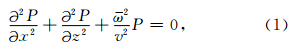
二维笛卡尔坐标系中的声波频率-空间域波动方程为
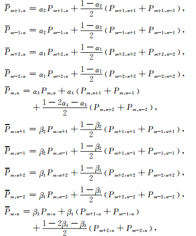
基于平均导数法(Chen, 2001,2008)我们推导出可适用于矩形网格和方形网格的四阶精度差分格式,其中加速度项采用Churl-Hyun等1996年提出的平均加速度项方法:
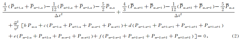
αi,βi,b,c,d,e和f为加权系数,b+4c+4d+4e+4f=1.差分格式如图 1所示.
 | 图 1 差分格式及系数分布示意图Fig. 1 Computational grid and coefficients of the 17-point scheme |
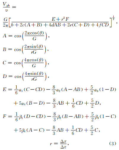
首先进行频散分析(详见附录A),可以得到归一化的相速度公式为
为了使得频散最小,我们构造如下目标函数:
优化过程中控制相速度相对误差在1%范围内,首先通过模拟退火法得到较好的初值,由于 MATLAB中fmincon函数提供了子空间信赖域的 大型优化方法,在初值附近泰勒展开,因此我们运用模拟退火法得到的初值用fmincon函数进一步优化(详见附录A),最终可以得到优化系数αi,βi,b,c,d,e,f,频散曲线如图 2所示,左半部分是传统9点四阶精度的频散曲线,右半部分是采用本文方法得到的频散曲线.我们仅给出r=dx/dz=1,1.5,2,2.5的频散曲线,更多不同r情形下的频散曲线可通过表 1和表 2中给出的优化系数得出. 通过表 1和2可以看出,在比率r相同时,dz>dx与dx>dz的优化系数b,c,d,e,f是相同的. 由图 2所示,在相速度相对误差1%范围内,本文方法单个波长所需的网格点只需2.4个,而传统9点四阶方法需要5个.
 | 图 2 不同r(r=Δx/Δz)时传统四阶9点格式和本文方法相速度频散曲线Fig. 2 Normalized phase velocity curves of the conventional fourth-order scheme and the adaptable 17-point scheme for different r=Δx/Δz |
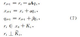
共轭梯度法(Hestenes and Stiefel, 1952)属于Krylov子空间类方法,对于大规模对称、正定、稀疏线性方程组是一种有效的迭代方法,Fletcher于1976年针对非对称系数矩阵提出双共轭梯度方法, van der Vorst(1992)在此基础上提出稳定双共轭梯度(BICGSTAB),其理论基础是双边Lanczos正交化方法(BICG)和广义共轭梯度平方法(CGS),比双共轭梯度法收敛更快、更平滑.
稳定双共轭梯度法的基本思想如下.
频率-空间域各向同性介质中Helmholtz 方程为
设xi是第i次迭代解,r i= s - A xi是残差量,r0与 0不正交,Ki(i维子空间)和i是分别与r0和0有关的量,通过下式寻找参数α,β.
一般情况下,频率域声波方程所形成的系数矩阵特征值变化范围大,条件数也较大,致使收敛性不好或者无法收敛,此时需要结合预处理技术,如不完全LU分解、不完全Cholesky分解、超松弛迭代、多重网格等加速收敛过程.不完全LU分解是一种通 用性很强的方法,由Meijerink和van der Vorst首 次提出(Meijerink and van der Vorst,1977). 将不 完全LU分解记做ILU(p),p的大小决定不完全 LU分解后引入填充量的多少,填充量越多和的稀疏性越低,计算量增加,但预处理效果越好. 兼顾预处理效果与计算效率,本文采用ILU(0),即在原矩阵零元素位置上将分解得到的非零元抛弃,如图 3所示.
 | 图 3 不完全LU分解后非零元素分布示意图.(b)(c)为(a)不完全分解后的矩阵Fig. 3 The non-zero elements after LU decomposition |
不完全LU分解的算法如下:
用相同的速度模型及参数测试稳定双共轭梯度方法及预条件稳定双共轭梯度方法,取误差限为1×10⁻¹⁰,从图 4可以看出,稳定双共轭梯度法在20000次仍未达到设定误差限,而预条件稳定双共轭梯度法在第6次迭代就已达到设定误差限.
预条件的共轭梯度等迭代法中除求解辅助性线性方程组外,其余主要是矩阵与向量乘操作,适合并行处理. 我们利用GPU强大的并行计算能力进行加速,CPU主要负责逻辑处理,GPU负责高度并行任务.在GPU上执行的称为内核函数(kernel),kernel内部是并行,各个kernel之间串行. CUDA中的基本逻辑执行单位是网格(grid)、线程块(block)、线程(thread)和线程组(warp),线程块是内核函数执行的基本单元,如图 5所示. NVIDIA研究团队2009年实现了稀疏矩阵向量乘的CUDA运算,并于2011年与EM Photonics 研究团队合作开发了CULA(基于GPU加速的线性代数库),对常用的迭代算法进行了加速,借助该线性代数库,分 别进行基于CPU平台和GPU协同计算平台的频 率-空间域正演单炮测试,测试机器处理器为i5-2320,内存8G,显卡为NVIDIA GeForce GTS 450,模型规模为500×500,取5次结果平均值作为运算时间,结果显示获得了1.5倍的加速比.
 | 图 4(a)速度模型;(b)稳定双共轭梯度法相对误差随迭代次数变化曲线;(c)不完全LU分解预条件稳定双共轭梯度法相对误差随迭代次数变化曲线Fig. 4(a)Velocity model;(b)The relative error cure of BICGSTA;(c)The relative error cure of BICGSTA with ILU for preconditioning |
 | 图 5 GPU组织结构和存储示意图Fig. 5 The structure and memory of GPU |
为了验证本文方法的精度,我们进行了与解析解的对比测试.
均匀介质中的解析公式(Alford et al., 1974)为
观测系统如图 6a所示,模型大小为50×50,dx=dz=15 m,震源采用雷克子波,边界条件采用完全匹 配层(PML)(详见附录C),层数为30. 解析解和本 文方法的单道记录如图 6b和6e所示.
 | 图 6(a)均匀模型的观测系统;(b)解析解单道记录;(c)9点格式的单道记录;(d)25点格式的单道记录;(e)本文方法的单道记录;(f)时间域有限差分单道记录Fig. 6(a)Geometry of the modeling;(b)The analytical solutions;(c)Numerical solutions of 9-point operator;(d)Numerical solutions of 25-point operator;(e)Numerical solutions of our 17-point scheme;(f)Numerical solutions of the time domain method |
 | 图 7计算时间对比示意图(纵坐标为归一化结果)Fig. 7 Computing time tested by our 17-point scheme,the 25-point scheme and the 9-point scheme |
 | 图 8内存占用对比示意图(纵坐标为归一化结果)Fig. 8 Memory usage by the 9-point scheme,our 17-point scheme and the 25-point scheme |
 | 图 9 (a)Marmousi模型示意图;(b)本文方法正演结果;(c)时间域有限差分正演结果Fig. 9(a)The Marmousi model;(b)Time-domain seismograms computed with the 17-point scheme;(c)Seismograms obtained by time-domain method |
我们选择有代表性的方法与本文方法进行相同测试条件下精度和计算效率的对比测试. Churl-Hyun等(1996)提出的9点格式是基于旋转坐标系的经典方法,现在仍广泛使用,后期很多方法也是基于其思想发展而来. Shin和Sohn于1998年首次提出四阶精度的方法,这两种方法发展较早且知名度较高,因此我们选择与其进行对比测试. 为了验证频率域正演的正确性,我们还给出了相同测试条件下的时间域有限差分的结果,时间域方法采用时间二阶差分、空间十阶差分,边界采用PML,结果如图 6f所示,通过与9点和25点方法对比可以看出本文方法在精度上具有优势.
本文介绍的方法中计算一点的导数用到的网格点比9点格式(Churl-Hyun et al., 1996)要多,因此在计算效率上需要进一步分析,为此我们进行了与9点格式(Churl-Hyun et al., 1996)、25点格式(Shin and Sohn, 1998)的对比测试. 模型大小为 300×300,速度为2000 m·s-1,采样间隔dx=dz=25 m,子波采用主频为20 Hz的雷克子波.为排除其他因素干扰,我们采用无边界条件进行测试,测试机器的处理器主频为3.00 GHz,内存为8 GB. 本文方法由于单波长只需要2.4个网格点就能达到1%相对误差,因此如果达到相同的正演精度,9点格式方法需要nx×nz个网格点,本文方法仅需(2.4/4)nx×(2.4/4)nz个网格点,25点方法则需要(2.5/4)nx×(2.5/4)nz个网格点,进行对比的测试结果如图 7所示.达到相同的精度,本文方法所需的网格点数较少,导致内存占用量也较少.稀疏矩阵的存储主要和非零元素有关,按照上文假设,如果9点格式方法需要nx×nz个网格点,则系数矩阵非零元素的个数为9×(nx×nz)2,25点格式方法为25×(2.5/4)(2.5/4)(nx×nz)2=9.76×(nx×nz)2,而本文方法的存储量为17×(2.4/4)(2.4/4)(nx×nz)2=6.12×(nx×nz)2,如图 8所示. 5 理论模型测试
为了进一步说明本算法适用于矩形网格,我们对Marmousi模型进行了地震波场正演模拟计算,如图 9所示为Marmousi速度模型.x方向采样间隔为12.5 m,z方向为4 m,频率域正演时子波采用雷克子波,主频为7 Hz,时间采样间隔为0.01 s,PML层数为40. 作为对比,进行了相同条件下时间域有限差分的测试,离散采用时间二阶空间十阶,子波与频率域方法相同,时间采样间隔是0.5 ms,同样是PML边界,层数为40.
如图 9所示,本文方法与时间域方法正演模拟结果一致,说明本文方法在矩形网格情形下是适用的,而传统的9点格式和25点格式的方法则不适用.鉴于在相速度相对误差1%范围内,本文提出的差分算子单个波长所需的网格点只需2.4个,因此对于同样面积的区域正演模拟,该方法可以使用较其他方法更粗的网格达到所需的正演模拟精度,大大减少了计算规模,如果是三维情形下,计算规模减少的更多.另外,结合本文提出的GPU加速迭代法,进一步提高了正演模拟的效率,为进行三维实际地质模型正演模拟打下基础. 6 结论
本文介绍了一种较传统算法适应范围更广、计算效率更高的频率-空间域正演方法. 通过采用平均导数法,使得该方法适用于方形网格和矩形网格,拓宽了原有传统方法的适用范围. 通过优化差分系数,使得单个波长所需网格点数减少到2.4.与解析解、9点格式、25点格式的均匀介质单道记录对比,可以看出本文方法在精度上具有优势,同样在计算效率与存储方面也优于9点和25点格式方法.为了避免Helmholtz方程直接法求解的困难,本文使用了迭代算法,结合不完全LU分解预条件,可以使得稳定双共轭梯度法加速收敛,进一步借助GPU协同计算,加速了本文算法中矩阵向量乘的计算,取得了较好的加速效果. 附录A
把平面波方程P(x,z)=P0e-i(kxx+kzz)代入公式(2)中得到
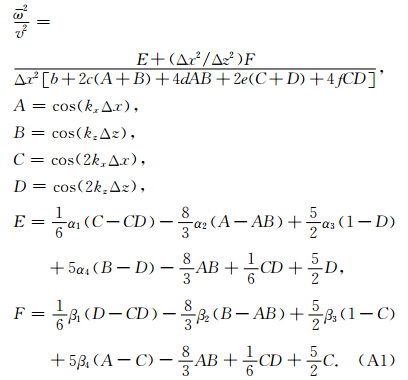
分两种情况讨论,当dx≥dz时,根据相速度定义 ,得到
,得到
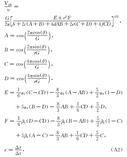
通过模拟退火法可以得到优化系数,但该优化系数并不能满足需要,进一步把上述优化系数作为初始迭代值,通过MATLAB中有约束非线性优化函数fmincon可以得到频散更小的优化系数,结果如表 1所示.
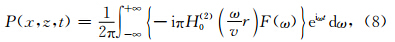
当dx 此处G=λ/Δz. 对于线性方程组 首先计算 判断i≤Iteration_max & error≥Error_max,如果为真,结束迭代,如果为假,继续; 令ρi-1= 若i=1,则qi=ri-1; 否则,计算βi-1=(ρi-1/ρi-2)(αi-1/ωi-1),qi=ri-1+βi-1(qi-1-ωi-1vi-1); 计算FM 如果error=‖g‖<Error_max,xi=xi-1+αi 否则,计算 继续判断i≤Iteration_max & error≥Error_max,后续重复上述步骤. 附录C PML边界的频率域声波方程(Berenger,1994)为 本文方法的有限差分方程可写为 


 ,q0=0,v0=0;
 =qi,vi=Aq,αi=βi-1/(,得到结果xi;
| [1] | Alford R M, Kelly K R, Boore D M. 1974. Accuracy of finite-difference modeling of the acoustic wave equation. Geophysics, 39(6):834-842, doi:10.1190/1.1440470. |
| [2] | Berenger J P. 1994. A perfectly matched layer for the absorption of electromagnetic waves. Journal of Computational Physics, 114(2):185-200, doi:10.1006/jcph.1994.1159. |
| [3] | Cao S H, Chen J B. 2012. A 17-point scheme and its numerical implementation for high-accuracy modeling of frequency-domain acoustic equation. Chinese J. Geophys. (in Chinese), 55(10):3440-3449, doi:10.6038/j.issn.0001-5733.2012.10.027. |
| [4] | Churl-Hyun J, Shin C, Suh J H. 1996. An optimal 9-point, finite-difference, frequency-space, 2-D scalar wave extrapolator. Geophysics, 61(2):529-537, doi:10.1190/1.1443979. |
| [5] | Chen J B. 2001. New schemes for the nonlinear Shrödinger equation. Applied Mathematics and Computation, 124(3):371-379, doi:10.1016/S0096-3003(00)00111-9. |
| [6] | Chen J B. 2008. Variational integrators and the finite element method. Applied Mathematics and Computation, 196(2):941-958, doi:10.1016/j.amc.2007.07.028. |
| [7] | Chen J B. 2012. An average-derivative optimal scheme for frequency-domain scalar wave equation. Geophysics, 77(6):T201-T210, doi:10.1190/geo2011-0389.1. |
| [8] | Chen J B. 2013. A generalized optimal 9-point scheme for frequency-domain scalar wave equation. Journal of Applied Geophysics, 92:1-7, doi:10.1016/j.jappgeo.2013.02.008. |
| [9] | Chen J B. 2014. Dispersion analysis of an average-derivative optimal scheme for Laplace-domain scalar wave equation. Geophysics, 79(2):T37-T42, doi:10.1190/geo2013-0230.1. |
| [10] | Chu C L, Stoffa P L. 2012. An implicit finite-difference operator for the Helmholtz equation. Geophysics, 77(4):T97-T107, doi:10.1190/geo2011-0314. 1. |
| [11] | Erlangga Y A. 2008. Advances in iterative methods and preconditioners for the Helmholtz equation. Archives of Computational Methods in Engineering, 15(1):37-66, doi:10.1007/s11831-007-9013-7. |
| [12] | Fletcher R. 1976. Conjugate gradient methods for indefinite systems.//Proceedings of the Dundee Conference on Numerical Analysis. Lecture Notes in Mathematics. Berlin Heidelberg:Springer, 506:73-89, doi:10.1007/bfb0080116. |
| [13] | Gu B L, Liang G H, Li Z Y. 2013. A 21-point finite difference scheme for 2D frequency-domain elastic wave modelling. Exploration Geophysics, 44(3):156-166, doi:10.1071/EG12064. |
| [14] | Hestenes M R, Stiefel E L. 1952. Methods of conjugate gradients for solving linear systems. J. Res. Nat. Bur. Standards Section B, 49(6):409-436. |
| [15] | Liu L, Liu H, Liu H W. 2013. Optimal 15-point finite difference forward modeling in frequency-space domain. Chinese J. Geophys. (in Chinese), 56(2):644-652, doi:10.6038/cjg20130228. |
| [16] | Luo Y, Schuster G. 1990. Parsimonious staggered grid finite-differencing of the wave equation. Geophysical Research Letters, 17(2):155-158, doi:10.1029/GL017i002p00155. |
| [17] | Meijerink J A, van der Vorst H A. 1977. An iterative solution method for linear systems of which the coefficient matrix is a symmetric M-matrix. Mathematics of Computation, 31:148-162, doi:10.1090/S0025-5718-1977-0438681-4. |
| [18] | Min D J, Shin C, Kwon B D, et al. 2000. Improved frequency-domain elastic wave modeling using weighted-averaging difference operators. Geophysics, 65(3):884-895, doi:10.1190/1.1444785. |
| [19] | Operto S, Virieux J, Amestoy P, et al. 2007. 3D finite-difference frequency-domain modeling of visco-acoustic wave propagation using a massively parallel direct solver:A feasibility study. Geophysics, 72(5):SM195-SM211, doi:10.1190/1.2759835. |
| [20] | Plessix R E. 2007. A Helmholtz iterative solver for 3D seismic-imaging problems. Geophysics, 72(5):SM185-SM194, doi:10.1190/1.2738849. |
| [21] | Plessix R E. 2009. Three-dimensional frequency-domain full-waveform inversion with an iterative solver. Geophysics, 74(6):WCC149-WCC157, doi:10.1190/1.3211198. |
| [22] | Pratt R G, Worthington M H. 1990. Inverse theory applied to multi-source cross-hole tomography. Part I:Acoustic wave-equation method. Geophysical Prospecting, 38(3):287-310, doi:10.1111/j.1365-2478.1990.tb01846.x. |
| [23] | Riyanti C D, Erlangga Y A, Plessix R E, et al. 2006. A new iterative solver for the time-harmonic wave equation. Geophysics, 71(5):E57-E63, doi:10.1190/1.2231109. |
| [24] | Shin C, Sohn H. 1998. A frequency-space 2-D scalar wave extrapolator using extended 25-point finite-difference operator. Geophysics, 63(1):289-296, doi:10.1190/1.1444323. |
| [25] | Shin C, Cha Y H. 2008. Waveform inversion in the Laplace domain. Geophysical Journal International, 173(3):922-931, doi:10.1111/j.1365-246X. 2008.03768.x. |
| [26] | Štekl I, Pratt R G. 1998. Accurate viscoelastic modeling by frequency-domain finite differences using rotated operators. Geophysics, 63(5):1779-1794, doi:10.1190/1.1444472. |
| [27] | Tarantola A. 1984. Inversion of seismic reflection data in the acoustic approximation. Geophysics, 49(8):1259-1266, doi:10.1190/1.1441754. |
| [28] | van der Vorst H A. 1992. Bi-CGSTAB:a fast and smoothly converging variant of bi-CG for the solution of nonsymmetric linear systems. SIAM J. Sci. Stat. Comput., 13(2):631-644, doi:10.1137/0913035. |
| [29] | Virieux J, Operto S. 2009. An overview of full-waveform inversion in exploration geophysics. Geophysics, 74(6):WCC1-WCC26, doi:10.1190/1.3238367. |
| [30] | 曹书红, 陈景波. 2012. 声波方程频率域高精度正演的17点格式及数值实现. 地球物理学报, 55(10): 3440-3449, doi: 10.6038/j.issn.0001-5733.2012.10.027. |
| [31] | 刘璐, 刘洪, 刘红伟. 2013. 优化15点频率-空间域有限差分正演模拟.地球物理学报, 56(2): 644-652, doi: 10.6038/cjg20130228. |