 2015, Vol. 58


2. 武汉大学测绘学院, 武汉 430079
2. School of Geodesy and Geomatics, Wuhan University, Wuhan 430079, China
The theoretical basis for Te estimating is the flexural isostatic model. Te can be established by minimizing the RMS misfit between the observed and theoretical admittance. The theoretical admittance is calculated based on flexural isostatic model. The observed admittance is calculated based on cross-spectral analysis of bathymetry and gravity model. We can calculate Te in two steps. First, at 20~50 km wave bands, the uncompensated theoretical admittance is calculated with different ρc (2300~2900 kg·cm3) and d (mean model depth ±500 m). The value of ρc and d can be recovered area by area by fitting the theoretical and observed admittance. Secondly, at wave lengths longer than 50 km, with the recovered ρc and d, the theoretical admittance can be computed for different Te. We can obtain an optimal Te when the RMS misfit between the theoretical and observed admittance is minimized. With the MWAT method, six windows range from 400 km×400 km to 1400 km×1400 km are used to estimate Te, using 3D spectral analysis technique. The final Te is weighted mean of these six results. For comparison, three kinds of bathymetry model are used. They are GEBCO, SIO V15.1 and BAT_VGG. BAT_VGG is a bathymetry model formed with ship soundings and vertical gravity gradient anomalies.
In our simulations, Te centered on (21°N, 157°E) is recovered for different inputted Te (1~50 km). The effects of crustal density, Young's modulus and high order terms are evaluated. The simulated results shown that the accuracy of Te calculated with MWAT method is ±1 km for Te<5 km and the relative accuracy can be better than 10% for Te≥5 km.The spatial variations of Te in the Northwestern Pacific are evaluated based on BAT_VGG and altimetric gravity anomaly data from SIO V20.1, with MWAT method. In the Northwestern Pacific, the results show that Te is in the range of 0~50 km with a mean of 13.2 km and a standard deviation of 6.9 km. High Te (20~40 km) distributes around the Hawaiian Islands and along the trench outer rise. The trench outer rise has the oldest lithosphere in the studied region, and their rigidity may have been modified by the plates' collision too. Hawaiian-Emperor is an intraplate original Seamount Chain. High Te around Hawaiian Islands is consistent with their formation on old, strong oceanic lithosphere. Te decreases monotonically along the Hawaiian Islands from the south-east end to the north-west end. Te along the northern Emperor Seamounts varies less systematically. Lithosphere around Shatsky Rise has the lowest Te (<5 km). Shatsky Rise formed at the Pacific-Farallon-Izanagi triple junction during the Late Jurassic to Early Cretaceous. Magnetic lineations indicate that the lithosphere is young at the time of Shatsky Rise loading. Low Te is consistent with the age of lithosphere at time of loading indicated by magnetic lineations. A wide oceanic basin spread in the south of Hawaiian-Emperor Seamount Chain. The Jurassic lithosphere locates in the west of the basin and has moderate Te (10~15 km). In the east of the basin, the lithosphere is formed during Cretaceous and has lower Te (<10 km). In the studied area, the dependence of Te on the age of oceanic lithosphere at the time of loading is given mostly by the depth to the 150℃~450℃ oceanic isotherm based on a cooling plate model, slightly lower than the depth given by Watts (2001) which is 300℃~600℃. Te of the Cretaceous and Jurassic lithosphere distributes in the 150℃~300℃ isotherm depth. Te of the Cretaceous lithosphere is less than the Jurassic lithosphere. Te of the lithosphere does not increase with the age of lithosphere at the time of loading. The result indicates that Te does not controlled only by the age of lithosphere at the time of loading. The reheating of the lithosphere by thermal activities inner the earth, such as the "super swells" in the South Pacific Ocean, and modification of the lithosphere by fracture zones will decrease the strength of the lithosphere.
We can draw the following conclusions from this paper: ① The gravity isostatic admittance in 20~50 km wavelengths band will not change significantly with Te. The regional crustal density and mean water depth can be recovered based on the admittance at 20~50 km wavebands. ② The simulated results shown that the accuracy of Te calculated with MWAT method is ±1 km for Te<5 km and the relative accuracy can be better than 10% for Te≥5 km. ③ The bathymetry model predicted from VGG and ship soundings (BAT_VGG) is superior to GEBCO and SIO V15.1 in Te estimating. With BAT_VGG, the mean recovered crustal density is consistent with CRUST2.0. The mean of standard deviation of the misfits between observed and theoretical admittance is 5.233 mGal/km, and about 56.869% of the grids have the standard deviation which lower than 5 mGal/km. ④ The results show that Te is in range of 0~50 km with a mean of 13.2 km and a standard deviation of 6.9 km over the Northwestern Pacific. The lithosphere of Hawaiian-Emperor Chain show relatively high Te. ⑤ Over the Northwestern Pacific, the dependence of Te on the age of oceanic lithosphere at the time of loading is given mostly by the depth to the 150℃~450℃ oceanic isotherm based on a cooling plate model, slightly lower than the depth given by Watts (2001), which is 300℃~600℃.
1 引言
有效弹性厚度(Te,Effective Elastic Thickness)作为岩石圈强度的定量描述,定义为与岩石圈板块中实际应力分布所产生的弯矩(Bending Moment)相等的弯曲弹性薄板的厚度(Forsyth,1985; 焦述强和金振民,1996),标志着在地质时间尺度内,岩石圈承受超过100 MPa压力时,发生弹性行为和流体行为转变的深度(McNutt,1990; 付永涛等,2000).海底岩石圈Te是研究海山构造及演化的基础数据(Wessel and Lyons, 1997; Wessel,2001),能为岩石流变学研究提供独立约束(Watts and Zhong, 2000; Mei et al., 2010),并为定量研究海底岩石圈强度演化、标定其屈服强度和研究应力状态提供必要数据(付永涛等,2002; Watts et al., 2013).岩石圈有效弹性厚度计算结果,可为板块动力学模型的构建,岩石圈挠曲形变动力学机制等地球动力学研究提供依据,在油气资源勘探等应用上也具有重要意义.
海底岩石圈Te的计算方法可分为三类:正演法、反演法和导纳分析法.正演法是指根据海底地形数据,通过调整Te,计算不同参数下海底地形及其均衡补偿物质产生的重力异常、大地水准面或岩石圈挠曲量,并将正演计算值与观测值进行比较,当两者之差的均方根达到最小时,可以确定Te(Watts and Cochran, 1974; Calmant,1987; Calmant et al., 1990; Watts,1994; Luis et al., 1998).反演法是指根据重力异常/大地水准面数据,在不同有效弹性厚度参数下,反演计算海底地形,并将计算结果与海深观测值比较,当两者之差的均方根达到最小时,获得Te估值(Goodwillie and Watts, 1993; Lyons et al., 2000; Watts et al., 2006).导纳分析法是指在频域内对重力异常和海底地形数据进行谱分析,求得重力-地形导纳,将此实测导纳与根据岩石圈挠曲均衡模型获得的模型导纳进行比较,通过调整有效弹性厚度参数,使实测导纳和模型 导纳之差的均方根最小,从而对Te作出估计(Watts,1978; McNutt,1979; Luis and Neves, 2006).
在国外,自20世纪70年代起,学者们已计算了全球海山地区的大量岩石圈有效弹性厚度(Te),且统计表明,Te主要受控于岩石圈温度结构.以板块冷却模型(Cooling Plate Model)为参考(Parsons and Sclater, 1977; Stein and Stein, 1992),Te主要分布在300 ℃~600 ℃等温线深度范围内(Watts,2001),但是,这些计算结果大多针对特定地质体,采用的数据和方法均不统一,相互之间存在较大差异,难以用于构建海底岩石圈有效弹性厚度模型,限制了计算成果的应用与进一步深入研究.Kalnins和Watts提出采用统一数据和方法,计算海底岩石圈Te(Kalnins and Watts, 2009).他们首先采用高斯型海山模型,模拟分析了滑动窗口导纳分析法(MWAT:Moving Window Admittance Technique,分别对覆盖面积不等的输入数据进行三维导纳分析,计算有效弹性厚度,再将各计算值进行带权平均,求得最终计算结果)的计算精度,得出MWAT法计算结果较真值系统性偏小20%的结论,在此基础上,计算了西北太平洋及全球海底岩石圈有效弹性厚度模型.Kalnins和Watts的研究中存在两个问题:一是模拟研究中采用了高斯型海山模型,这与实际海底形态不符,且未分析洋壳密度、杨氏模量等参数影响;二是采用的海底地形要么是精度较低的GEBCO模型,要么是与重力异常直接相关的(15~160 km波段内根据重力异常反演计算)、来自斯克里普斯海洋研究所(SIO:Scripps Institute of Oceanography)的V15.1模型,因而Te计算结果精度和可靠性需进一步分析.Wang指出,根据垂直重力梯度异常反演计算的海底地形模型,不直接依赖于重力异常,可 能更适用于采用导纳分析法计算岩石圈Te(Wang,2000). 胡敏章(2014b)联合船测海深和垂直重力梯度异常数据,构建了全球海底地形模型(BAT_VGG),本文拟将该模型应用于计算Te,并将其与GEBCO和SIO V15.1模型进行对比分析.
在国内,直到20世纪90年代才开始关注岩石圈强度研究,且集中于研究中国大陆岩石圈有效弹性厚度及其构造意义(周辉,1997;付永涛,2000;袁炳强等,2002;赵俐红等,2004).近年来,对中国大陆岩石圈有效弹性厚度的研究,又陆续有新成果发表(郑勇等,2012;杨亭等, 2012,2013;李永东等,2013). 国内对海底岩石圈有效弹性厚度研究一直较少,从检索的文献看,仅有刘保华等(1998)对冲绳海槽地区岩石圈有效弹性厚度的探讨;付永涛等(2002)对大洋和大陆边缘岩石圈有效弹性厚度研究意义的综述性阐述;赵俐红等(2010)对中西太平洋个别海山区域岩石圈有效弹性厚度及其地质意义研究;以及苏达权(2012)采用三维导纳分析法估算了我国南海南沙海域和南海中央海盆岩石圈有效弹性厚度分别约为10 km和6~7 km.
本文以西北太平洋地区为例(145°E —215°E,15°S—45°N),首先,基于SIO V15.1模型,模拟分析了MWAT法的计算精度,研究了杨氏模量、洋壳密度等参数的影响;其次,分别采用GEBCO、SIO V15.1和BAT_VGG模型,利用MWAT法构建了研究区域的岩石圈有效弹性厚度,对三种情况下的Te计算结果进行了分析;然后,根据本文Te计算结果,结合收集到的海山和洋底年龄数据,分析了其构造成因. 2 岩石圈有效弹性厚度计算原理与数据 2.1 计算原理
岩石圈挠曲均衡理论是根据海底地形和重力异常计算Te的理论基础.根据挠曲均衡理论,在海山载荷作用下,洋壳将向下挠曲,如图 1所示,图中d为平均水深,t为平均洋壳厚度,h(x)为海山,r(x)为洋壳挠曲,ρm、ρc、ρw分别为地幔、洋壳和海水密度.
 | 图 1 海底岩石圈挠曲均衡模型 Fig. 1 Flexural isostatic model of the seafloor lithosphere |
根据Parker公式(Parker,1972),在频域内,海底地形与海面重力异常之间的关系为
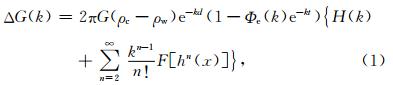
 ,E为杨氏模量,Te为岩石圈有效弹性厚度,υ为泊松比.Parker的研究表明,公式(1)收敛速度快,如果仅顾及n=1项,则可得海底地形与重力异常之间的导纳关系为

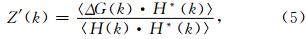
导纳分析法计算岩石圈有效弹性厚度的一般原理是:对重力异常和海底地形进行谱分析,计算两者之间的导纳关系,即“实测导纳” Z′(k),将计算结果与Te取不同值时,根据公式(4)计算的模型导纳进行比较,当两者之差的均方根最小时,获得Te计算结果.影响模型导纳的参数主要是洋壳密度ρc、平均水深d和Te,取表 1中参数,计算模型导纳如图 2所示.
 | 图 2 理论挠曲均衡模型的均衡重力模型导纳曲线 (a)不同Te值;(b)不同平均水深;(c)不同洋壳厚度. Fig. 2 Theoretical gravity admittance of flexural isostatic model (a)Different Te;(b)Different water depth;(c)Different crust density. |
|
|
表 1 理论挠曲均衡模型重力导纳计算的洋壳模型参数 Table 1 Theoretic parameters of ocean crust for flexural isostatic model |
采用表 1中的参数,当海山密度为2800 kg·m-3、 平均水深为4.5 km时,取Te分别为5 km、10 km、20 km、40 km时,模型导纳如图 2a所示;当取海山密度为2800 kg·m-3、Te为10 km,取平均水深为2 km、3 km、4.5 km、5.5 km时,模型导纳如图 2b所示;当取平均水深为4.5 km,Te为10 km时海山密度分别取2400 kg·m-3、2500 kg·m-3、2600 kg·m-3、2800 kg·m-3时,模型导纳如图 2c所示.从图 2a可以看出,岩石圈板块的有效弹性厚度主要影响波长大于50 km部分的模型导纳;从图 2b可知,平均水深主要影响波长小于100 km部分的模型导纳;从图 2c可知,海山密度的影响范围几乎是全波段的,其中对中间波段影响比较大.
实际Te计算过程中,计算模型导纳时,首先以20~50 km波段内实测导纳为约束,通过调整平均水深参数和洋壳密度参数计算模型导纳,当模型导纳与实测导纳之差的均方根最小时,获得平均水深和洋壳密度参数;然后,再以大于50 km部分的实测导纳为约束,通过调整有效弹性厚度参数,计算模型导纳,当两者之差的均方根最小时,确定有效弹性厚度Te.计算过程中,洋壳密度参数以CRUST2.0为参考,在2300~2900 kg·m-3范围内调整;平均水深参数以输入的海底地形水深平均值为参考,围绕该值在±300 m范围内调整.因此,在计算获得Te的同时,还可获得洋壳密度估值,此参数可以作为除实测导纳与模型导纳之差的均方根之外,评估计算结果可靠性的另一指标.
以三个计算点为例,来说明岩石圈有效弹性厚度的计算过程,分别为(a)皇帝海山(170°E,42°N)、(b)中太平洋海岭东部(172°W,18°N)和(c)麦哲伦海隆(Magellan Rise,177°W,7°N),数据取以此为中 心的800 km×800 km范围.模型导纳与实测导纳之差的均方根(RMS)随Te的变化如图 3所示.当均方根最小值分别为5.126 mGal/km、 2.569 mGal/km和4.104 mGal/km时,(a)、(b)、(c)三个计算点的岩石 圈有效弹性厚度分别为18.5 km、5.5 km和4.5 km. 模型导纳与实测导纳拟合情况如图 4所示.
 | 图 3 试算点模型导纳与实测导纳之差的均方根随Te的变化曲线 Fig. 3 The relationship between Te and the RMS of differences between observed and modeled admittance over the three experimental points |
 | 图 4 试算点模型导纳与实测导纳拟合情况(黑色点为实测导纳,虚线、点线和 点划线分别对应的是Te为最小估值、最佳估值和最大估值时的模型导纳) Fig. 4 The fitting between modeled and observed admittance over the three experimental points(the black dots denote the observed admittance,the dashed,dotted, and dotted-dashed lines denote admittances for the min,best, and max fitted Te respectively) |
图 4中,黑色点为根据重力异常和海底地形获得的实测导纳,点线为最佳拟合模型导纳,虚线和点划线为取模型导纳与实测导纳之差的均方根偏离最小值20%为阈值时,根据估算的最小和最大Te值计算的模型导纳. 2.2 数据
本文拟采用的重力异常来自SIO的卫星测高重力异常,版本V20.1(Sandwell and Smith, 2009).拟采用的海底地形模型包括GEBCO、SIO V15.1和BAT-VGG.GEBCO模型是根据数字化的海底等深线数据,联合少量船测海深数据构建的,精度较低(Goodwillie,2008).在西北太平洋(145°E—215°E,15°S—45°N),本节拟采用的海底地形模型与船测海深之差的统计参数见表 2.船测海深数据来 自美国国家地球物理数据中心(National Geophysical Data Center: NGDC). 海底地形的频率分布直方图如图 5所示.
 | 图 5 西北太平洋海底地形频率分布直方图 (a)GEBCO;(b)SIO V15.1;(c)BAT_VGG. Fig. 5 The frequency distribution histogram of bathymetry over the Northwestern Pacific (a)GEBCO;(b)SIO V15.1;(c)BAT_VGG. |
从表 2和图 5可以看出,GEBCO模型精度较低,且数据存在“阶梯”现象,即海深值在500 m的倍数上集中分布;SIO V15.1和BAT_VGG的精度和分布形态均优于GEBCO的.
|
|
表 2 海底地形模型与船测海深之差的统计(单位:m) Table 2 Statistics of the differences between bathymetry models and ship soundings in Northwest Pacific(Unit:m) |
本文从149°E—165°E,13°N—29°N实际海底 地形出发,分析MWAT法计算精度.采用 SIO V15.1模型,假定此地形为真值,分别在Te为1 km、 2 km、3 km、4 km、5 km、10 km、15 km、20 km、25 km、30 km、35 km、40 km、45 km和50 km时,根据公式(1),正演计算海底地形及其均衡补偿物质产生的重力异常,然后,联合正演重力异常与海底地形,采用MWAT法计算有效弹性厚度.模型中有效弹性厚度为确定值,因而可以分析多种参数对计算精度的影响.正演计算时洋壳模型参数如表 3所示.
|
|
表 3 正演计算时理论洋壳模型参数 Table 3 Theoretic ocean crust parameters of forward modeling |
模拟分析区域内有马尔库斯—威克平顶山群和麦哲伦海山链,海山分布较密集,海底地形与正演重 力异常(Te=10 km,公式(1)中取到n=4)如图 6所示.
 | 图 6 海底地形(a)与正演重力异常(b),取Te=10 km,n=4 Fig. 6 Seafloor topography(a) and forward modeled gravity anomalies(b)with Te=10 km and n=4 |
采用MWAT方法,窗口范围分别取400 km×400 km~1400 km×1400 km,间距为200 km,计算岩石圈有效弹性厚度.分别测试MWAT算法本身精度、重力异常数据中高次项影响、杨氏模量、洋壳密度参数对计算结果的不同影响,计算结果如图 7所示.
 | 图 7 模拟分析多种因素对Te计算值的影响 Fig. 7 Simulated analysis of influence of many factors for Te calculating |
图 7中,横坐标为真值,纵坐标为计算值,各符号对应不同参数设置情况下的计算结果,符号位于虚线下方表示计算结果较真值偏小,反之偏大.从图 7可以得到如下六点结论:① 符号“ ○ ”表示取公式(1)中n=1时正演重力异常进行Te计算,Te =5~35 km 时,计算值较真值平均偏小,约8.1%,Te大于35 km时计算偏差最大不超过5%.② 符号“Δ”表示公式(1)中n=4时高次项(n≥2)的影响,当Te为 20 km时,正演重力异常计算结果偏小,约12.6%;Te为25 km、30 km和35 km 时,平均偏小约6%;Te大于35 km时,计算偏差在5%以下.顾及正演重力异常高次项(n=4)时的Te计算结果与不顾及高次项(n=1)的计算结果,一般差距均在5%以内,说明重力异常中高次项(n≥2)对Te计算结果影响不大.③ 符号“ ◇ ”表示当E取值偏小值时(0.7×10¹¹N·m-2),Te计算结果偏大,Te真值为5~35 km时,平均偏大约4.4%.④ 符号“ □ ”,当密度参数偏小,为100 kg·m-3时,Te计算结果偏大,Te真值为5~35 km时,平均偏大约8.6%.⑤ 符号“ + ”,当密度参数偏大100 kg·m-3时,Te计算结果偏小,Te真值为5~35 km时,平均偏小约20.8%.可见,密度参数偏大的情况下,计算结果受影响最大,因此要尽量避免采用过大的洋壳密度参数.本文参考CRUST2.0模型参数,密度参 数取值范围限定在2300~2900 kg·m-3.⑥当Te<5 km时,无论何种情况下,Te计算误差均在±1 km以内;当Te≥ 40 km时,无论何种情况下,Te计算结果相对偏差不超过10%.只要不采用过大的洋壳密度参数,MWAT法计算Te的相对精度一般可保证在10%以内.
4 Te计算结果及其构造意义
4.1 计算结果 在研究区域(145°E—215°E,15°S—45°N),分别联合海底地形模型GEBCO、SIO V15.1、BAT_VGG与重力异常数据(来自SIO,版本V20.1),构建1°×1°岩石圈有效弹性厚度模型.共计算了4331个格网点的有效弹性厚度值,实测导纳与模型导纳之差的均方根(RMS)频率分布直方图如图 8所示.
 | 图 8 分别采用GEBCO(a)、SIO V15.1(b)和BAT_VGG(c)进行Te计算时模型导纳与实测导纳之差的均方根频率分布直方图 Fig. 8 RMS histogram of the differences between modeled admittance and observed admittance. Using different bathymetry models,(a)for GEBCO,(b)for SIO V15.1 and (c)for BAT_VGG |
Te计算过程中获得的洋壳密度参数平均值和标准差,以及模型导纳与实测导纳之差的均方根统计见表 4.
|
|
表 4 采用不同海底地形模型时洋壳密度参数和实测导纳与模型导纳之差的均方根统计 Table 4 Statistics of crust density and RMS of differences between modeled admittance and observed admittance when using different bathymetry models |
在研究区域,由CRUST2.0提供的洋壳密度平 均值为2772 kg·m-3,从表 4可以看出,采用BAT_VGG 模型进行Te计算时,洋壳密度平均值为2770 kg·m-3,与CRUST2.0的一致,且模型导纳与实测导纳之差的均方根平均值最小,56.869%计算点的均方根在5 mGal/km以内.
从图 8和表 4看,岩石圈有效弹性厚度计算时,BAT_VGG模型优于其他两个模型.
联合BAT_VGG海底地形模型(图 9a)与重力异常SIO V20.1(图 9b),采用MWAT法,计算获得研究区域岩石圈有效弹性厚度模型如图 10所示.
图 10中等值线是来自Müller等(2008)的岩石圈年龄数据,单位为Ma.在西北太平洋地区,岩石 圈有效弹性厚度的均值为13.2 km,标准差为6.9 km,从图 10可知,其分布有如下特点:①西部海沟地区和夏威夷群岛地区Te为20 km以上高值区;②夏威夷—皇帝海山链的岩石圈有效弹性厚度呈自东南至西北逐渐减小趋势;③洋盆区域岩石圈有效弹性厚度总体呈西高东低趋势,西部侏罗纪时期的岩石圈有效弹性厚度一般为10~15 km,中太平洋海岭和莱恩海岭地区的白垩纪时期岩石圈有效弹性厚度略小,一般为5~10 km;④沙茨基海隆地区岩石圈强度较弱,有效弹性厚度在5 km以下.
 | 图 9 研究区域的海底地形(a)和重力异常(b) SR:沙茨基海隆,HR:赫斯海隆,HE:夏威夷—皇帝海山链,MPM:中太平洋海岭,MW:马尔库斯—威克平顶山群,MI:马绍尔 群岛,GR:吉尔伯特海山链,LI:莱恩群岛,OJP:翁通爪哇海底高原,MP:马尼希基海底高原;红色虚线为断裂带,MeFZ:门多西诺 断裂带,MuFZ:默里断裂带,MoFZ:莫洛凯断裂带,ClaFZ:克拉里昂断裂带,CliFZ:克里帕顿断裂带,GFZ:加拉帕戈斯断裂带. Fig. 9 Bathymetry(a) and gravity anomalies(b)over the studied region SR: Shatsky Rise; HR: Hess Rise; HE: Hawaii-Emperor Seamounts; MPM: Mid-Pacific Mountains; MW: Marcus-Wake Guyots; MI: Marshall Isl and s; GR: Gilbert Rise; LI: Line Isl and s; OJP: OntongJava Plateau; MP: Manihiki Plateau; the red dashed lines denote fracture zones: MeFZ: Mendocino Fracture Zone; MuFZ: Murray Fracture Zone; MoFZ: Molokai Fracture Zone; ClaFZ: Clarion Fracture Zone; CliFZ: Clipperton Fracture Zone; GFZ: Galapagos Fracture Zone. |
 | 图 10 研究区域内,联合BAT_VGG与重力异常SIO V20.1计算的岩石圈有效弹性厚度(等值线根据文献(Müller et al., 2008)给出的海底岩石圈年龄绘制,单位Ma) Fig. 10 Lithospheric effective elastic thickness over the Northwestern Pacific(Contours for ocean lithospheric age based on literature(Müller et al., 2008),Unit: Ma) |
夏威夷-皇帝海山链是热点活动成因海山链,“热点”现位于岛链东南端,自东南至西北方向,海山年龄逐渐增大,海山加载时岩石圈年龄逐渐减小,因而岩石圈有效弹性厚度逐渐减小.沙茨基海隆形成于“三联点”活动,处于Airy均衡状态(Sandwell and MacKenzie, 1989; 胡敏章等,2014a),其岩石圈有效弹性厚度计算结果在5 km以下是合理的.研究区域的其他海山链,如莱恩海岭、中太平洋海岭等地区岩石圈有效弹性厚度,并未如夏威夷—皇帝海山链一样呈渐变趋势,可能反映它们经历了与夏威夷皇帝海山链不一样的演化过程.
Watts等(2006)采用“海底地形反演方法”计算了全球大量海山岩石圈有效弹性厚度,其中,在本文研究范围内,共有3095个岩石圈有效弹性厚度计算 结果,本文计算结果与Watts计算结果之差,如图 11所示.
 | 图 11 本文Te计算结果与Watts等计算结果之差 Fig. 11 Te differences between Watts et al. and this paper′s result |
从图 11可知,本文计算结果与Watts等计算结 果之差,约51.5%在±5 km以内,约79.5%在±10 km 以内,均值为-3.7 km,标准差为6.4 km,差距较大的点主要集中分布在夏威夷群岛周围.总体上,两种方法计算获得的结果一致性较好.与MWAT法相比,Watts等采用的方法有两大不足:① 它以船测海深数据为约束,这使得该方法仅适用于有足够船测海深数据覆盖的海山地区,而这部分面积占整个大洋的较小部分;② 它逐个计算独立海山下岩石圈有效弹性厚度,未能顾及海山周边地形的影响.MWAT法可以以统一的精度计算覆盖全球大洋的岩石圈有效弹性厚度模型,不再拘泥于海山地区,不依赖于船测海深数据的分布状况. 4.2 有效弹性厚度与海山加载时岩石圈年龄的关系
大洋岩石圈有效弹性厚度与岩石圈温度结构密切相关,根据板块冷却模型(Parsons and Sclater, 1977; Stein and Stein, 1992),岩石圈在洋中脊形成,随着板块扩张活动,逐渐冷却、下沉,强度增大.已有研究表明,Te一般分布于450 ℃±150 ℃等温面深度范围内,因此,根据Te计算结果,在已知洋底或海山年龄情况下,可以推测海山或洋底年龄(Calmant et al., 1990).
本文在西北太平洋地区的主要海山链上共收集了71个海山年龄数据(Schlanger et al., 1984; Calmant et al., 1990; Caplan-Auerbach et al., 2000; Clouard and Bonneville, 2001; Davis et al., 2002; Sharp and Clague, 2006),海山底部岩石圈年龄由岩石圈年龄数据库内插获得(Müller et al. 2008).岩石圈年龄减去海山年龄即是海山加载时岩石圈年龄.海山底部岩石圈有效弹性厚度如图 12所示.从图 12可以看出,夏威夷海山链的岩石圈有效弹性厚度总体呈从东南至西北方向逐渐减小趋势.莱恩海岭岩石圈有效弹性厚度无明显趋势性变化,约为10 km.马绍尔—吉尔伯特海山链岩石圈有效弹性厚度也无明显趋势性变化,一般为10~15 km.在马尔库斯—威克平顶山—中太平洋海岭一线,自西向东,岩石圈有效弹性厚度逐渐减小,这与岩石圈年龄呈减小趋势相符.
 | 图 12 海山链上的有效弹性厚度 Fig. 12 Te on seamounts |
以板块冷却模型(Plate Cooling Model)为参 考,绘制海山加载时岩石圈年龄与岩石圈有效弹性厚度关系图,如图 13所示.
 | 图 13 Te与海山加载时岩石圈年龄的关系(P & S:Parsons和Sclater给出板块冷却模型;GDH1:Stein和Stein给出的板块冷却模型;蓝色三角形为夏威 夷—皇帝海山链上海山;红色圆点为侏罗纪时期形成的岩石 圈上海山; 紫色方形表示白垩纪时期形成的岩石圈) Fig. 13 Relationship between Te and age of oceanic lithosphere at time of loading(P & S: Plate cooling model given by Parsons and Sclater; GDH1: Plate cooling model given by Stein and Stein; the blue triangulars indicate seamounts on the Hawaii-Emperor Seamounts; the red circles denote seamounts on the Jurassic lithosphere; the purple squares denote seamounts on the Cretaceous lithosphere) |
从图 13可以看出,西北太平洋地区岩石圈有效弹性厚度主要分布在150 ℃~450 ℃等温面深度范围内,小于全球统计结果的等温面300 ℃~600 ℃.白垩纪时期形成的岩石圈有效弹性厚度一般小于侏罗纪时期岩石圈的.此外,从图 13可知,除夏威夷—皇帝海山链外,侏罗纪和白垩纪岩石圈有效弹性厚度并未随海山加载时岩石圈年龄增大而增大.可见,海山加载时岩石圈年龄不是影响研究区域岩石圈有效弹性厚度的唯一因素.对研究区海山岩性和形成年代的研究表明,本地区大量海山可能形成于现今南太平洋法属波利尼西亚地区,是白垩纪超级海隆活动的产物(初凤友等,2005;赵俐红等,2005).大规模的热活动,减小了岩石圈热年龄,使得其强度减弱了.研究区域还广泛分布有断裂带,这些断裂带对海底的改造作用,不仅影响了本地区海山分布形态,同时也会降低岩石圈强度(章家保等,2006;Farrar and Dixon, 1981; Nakanishi,1993). 5 讨论和结论
本文的研究还有两个方面需要探讨,一是沉积层等洋壳密度异常对Te计算的影响,二是大规模海山/海岛对Te计算的影响.由于当前对海底沉积层等密度异常分布的了解非常有限,在Te计算之前将其影响予以剔除是不可能的,但我们可以从洋壳模型上对其影响略加分析.本文在Te计算过程中采用了如图 1所示的简单洋壳模型,但实际洋壳密度结构要复杂得多,海山与其下洋壳密度可以不同,海山周围凹陷区域的沉积填充物密度(ρinfill)与海山密度(ρload)也可以不同,地震波速度结构也告诉我们,洋壳具有分层密度结构,因此可以构建更复杂的洋壳模型.作者构建了双层洋壳模型,经实际计算表明其理论导纳与图 1所示的单层模型差别很小.因此本文采用单层洋壳模型是可行、有效的.此外,大洋地区沉积层厚度一般很薄(0~0.5 km)(Divins,2003),因而对Te计算结果不会产生剧烈影响,更不会改变洋底岩石圈有效弹性厚度的变化趋势.
研究区域内最大的海山/海岛载荷为夏威夷群岛,GTR(Geoid Topography Ratio)研究表明,它处于Airy均衡状态(Sandwell and MacKenzie, 1989).在夏威夷群岛作用下,周边岩石圈发生挠曲形变,这可能影响Te计算结果.本文计算过程中,当实测导纳与模型导纳拟合效果不佳时,计算结果将被抛弃,图 10中展示的结果就剔除了夏威夷群岛东南部部分数据.MWAT法在夏威夷岛周边个别地区的应用上存在局限性,但在整个夏威夷海山链 上计算的Te变化趋势与文献Watts和Brink(1989),以及Wessel(1993)的较为一致.
本文的研究可得到如下结论:
①20~50 km波段内的均衡重力导纳基本不受有效弹性厚度影响,首先可以以此为约束,获得适合于计算区域的洋壳平均密度和平均水深参数,且需注意,密度参数不宜过大,本文参考CRUST2.0 模型,将洋壳密度参数限定在2300~2900 kg·m-3.
② 模拟研究表明,MWAT法计算岩石圈有效弹性厚度的精度较高:Te<5 km时,精度为±1 km,Te≥5 km 时,相对精度可达10%.
③ 进行岩石圈有效弹性厚度计算时,海底地形模型BAT_VGG优于SIO V15.1和GEBCO模型.采用BAT_VGG时,计算获得的洋壳密度参数平均值与CRUST2.0一致,且实测导纳与模型导纳之差的均方根更小,平均值为5.233 mGal/km,研究区域内56.869%的Te计算点的均方根在5 mGal/km以内.
④ 计算结果表明,西北太平洋地区岩石圈有效弹性厚度为0~50 km,均值为13.2 km,标准差为6.9 km.在夏威夷—皇帝海山,岩石圈有效弹性厚度较大(一般>20 km),且自西北至东南呈逐渐增大趋势;在中太平洋海岭、莱恩海岭等区域,岩石圈有效弹性厚度较小(一般<10 km);在西部的马尔库斯—威克平顶山、马绍尔群岛、吉尔伯特群岛等地区岩石圈有效弹性厚度大小适中(10~15 km).
⑤ 以板块冷却模型为参考,西北太平洋岩石圈有效弹性厚度总体上分布在150 ℃~450 ℃等温线深度范围内,小于全球统计的等温线范围结果300 ℃~600 ℃. 并且,夏威夷—皇帝海山链以南,白垩纪和侏罗纪时期的岩石圈有效弹性厚度大多分布于150 ℃~300 ℃等温线深度范围内,且未随海山加载时岩石圈年龄增大而增大,说明海山加载时岩石圈年龄不是影响岩石圈强度的唯一因素.白垩纪时期南太平洋超级海隆活动,以及研究区域广泛存在的断裂带活动,都曾对本地区岩石圈演化产生过重要影响.超级海隆活动使得岩石圈热年龄减小,降低了它的力学强度,而断裂带可能对研究区域海山分布形态有重要影响.
| [1] | Calmant S. 1987. The elastic thickness of the lithosphere in the Pacific Ocean. Earth Planet. Sci. Lett., 85(1-3): 277-288. |
| [2] | Calmant S, Francheteau J, Cazenave A. 1990. Elastic layer thickening with age of the oceanic lithosphere: a tool for prediction of the age of volcanoes or oceanic crust. Geophys. J. Int., 100(1): 59-67. |
| [3] | Caplan-Auerbach J, Duennebier F, Ito G. 2000. Origin of intraplate volcanoes from guyot heights and oceanic paleodepth. J. Geophys. Res., 105(B2): 2679-2697. |
| [4] | Chu F Y, Chen J L, Ma W L, et al. 2005. Petrologic characteristics and ages of basalt in middle Pacific Mountains. Marine Geology & Quaternary Geology (in Chinese), 25(4): 55-59. |
| [5] | Clouard V, Bonneville A. 2005. Ages of seamounts, islands and plateaus on the Pacific plate. GSA Special Papers, 388: 71-90. |
| [6] | Davis A S, Gray L B, Clague D A, et al. 2002. The Line Islands revisited: New 40Ar/39Ar geochronologic evidence for episodes of volcanism due to lithospheric extension. Geochem. Geophys. Geosyst., 3(3): 1-28, doi: 10.1029/2001GC000190. |
| [7] | Divins D L. 2003. Total Sediment Thickness of the World's Oceans & Marginal Seas. NOAA National Geophysical Data Center. Washington: NASA. |
| [8] | Farrar E, Dixon J M. 1981. Early tertiary rupture of the Pacific plate: 1700 km of dextral offset along the Emperor trough-Line Islands lineament. Earth Planet Sci. Lett., 53(3): 307-322. |
| [9] | Forsyth D W. 1985. Subsurface loading and estimates of the flexural rigidity of continental lithosphere. J. Geophys. Res., 90(B14): 12623-12632. |
| [10] | Fu Y T. 2000. Preliminary research on the lithospheric effective elastic thickness of Dabie Mountain. Beijing: Institute of Geology and Geophysics, Chinese Academy of Sciences. |
| [11] | Fu Y T, Li J L, Zhou H, et al. 2000. Comments on the effective elastic thickness of continental lithosphere. Geological Review (in Chinese), 46(2): 149-159. |
| [12] | Fu Y T, Li A C, Qin Y S. 2002. Effective elastic thickness of the oceanic and continental marginal lithospheres. Marine Geology & Quaternary Geology (in Chinese), 22(3): 69-75. |
| [13] | Goodwillie A M, Watts A B. 1993. An altimetric and bathymetric study of elastic thickness in the central Pacific ocean. Earth Planet. Sci. Lett., 118(1-4): 311-326. |
| [14] | Goodwillie A M. 2008. User guide to the GEBCO one minute grid. (http://www.gebco.net). |
| [15] | Hu M Z, Li J C, Li H, et al. 2014a. 3D admittance analysis for gravity isostasy on Shatsky Rise. Journal of Geodesy and Geodynamics (in Chinese), 34(2): 14-18. |
| [16] | Hu M Z, Li J C, Xing L L. 2014b. Global bathymetry model predicted from vertical gravity gradient anomalies. Acta Geodaetica et Cartographica Sinica (in Chinese), 43(6): 558-565, 574. |
| [17] | Jiao S Q, Jin Z M. 1996. Effective elastic thickness of continental lithosphere and its geodynamical significance. Geological Science and Technology Information (in Chinese), 15(2): 8-12. |
| [18] | Kalnins L M, Watts A B. 2009. Spatial variations in effective elastic thickness in the Western Pacific Ocean and their implications for Mesozoic volcanism. Earth Planet. Sci. Lett., 286(1): 89-100, doi: 10.1016/j.epsl.2009.06.018. |
| [19] | Li Y D, Zheng Y, Xiong X, et al. 2013. Lithospheric effective elastic thickness and its anisotropy in the northeast Qinghai-Tibet plateau. Chinese Journal of Geophysics (in Chinese), 56(4): 1132-1145, doi: 10.6038/cjg20130409. |
| [20] | Liu B H, Liu Z C, Wang S G. 1998. Preliminary study on the compensation model of submarine topography in the Okinawa Trough. Marine Geology & Quaternary Geology (in Chinese), 18(4): 29-34. |
| [21] | Luis J F, Miranda J M, Galdeano A, et al 1998. Constraints on the structure of the Azores spreading center from gravity data. Mar. Geophys. Res., 20(3): 157-170. |
| [22] | Luis J F, Neves M C. 2006. The isostatic compensation of Azores Plateau: a 3D admittance and coherence analysis. Journal of Volcanology and Geothermal Research, 156(1-2): 10-22. |
| [23] | Lyons S N, Sandwell D T, Smith W H F. 2000. Three-dimensional estimation of elastic thickness under the Louisville Ridge. J. Geophys. Res., 105(B6): 13239-13252. |
| [24] | Müller R D, Sdrolias M, Gaina C, et al. 2008. Age, spreading rates, and spreading asymmetry of the word's ocean crust. Geochem. Geophys. Geosyst., 9(4), doi: 10.1029/2007GC001743. |
| [25] | McNutt M. 1979. Compensation of oceanic topography: An application of the response function technique to Surveyor area. J. Geophys. Res., 84(B13): 7589-7598. |
| [26] | McNutt M. 1990. Flexure reveals great depth. Nature, 343(6259): 596-597. |
| [27] | Mei S, Suzuki M A, Kohlstedt D L, et al. 2010. Experimental constraints on the strength of the lithospheric mantle. J. Geophys. Res., 115(B8), doi: 10.1029/2009 JB006873. |
| [28] | Nakanishi M. 1993. Topographic expression of five fracture zones in the northwestern Pacific Ocean. //Pringle M S, Sager W W, Sliter W V, et al. The Mesozoic Pacific: Geology, Tectonics and volcanism. USA, John Wiley & Sons, Inc, 77: 121-136. |
| [29] | Parker R L. 1973. The rapid calculation of potential anomalies. Geophys. J. R. Astr. Soc., 31(4): 447-455. |
| [30] | Parsons R L, Sclater J G. 1977. An analysis of the variation of ocean floor bathymetry and heat flow with age. J. Geophys. Res., 82(5): 803-827. |
| [31] | Sandwell D T, MacKenzie K R. 1989. Geoid height versus topography for oceanic plateaus and swells. J. Geophys. Res., 94(B6): 7403-7418. |
| [32] | Sandwell D T, Smith W H F. 2009. Global marine gravity from retracked Geosat and ERS-1 altimetry: Ridge segmentation versus spreading rate. J. Geophys. Res., 114(B1), doi: 10.1029/2008JB006008. |
| [33] | Schlanger S O, Garcia M O, Keating B H, et al. 1984. Geology and geochronology of the line islands. J. Geophys. Res., 89(B13): 11261-11272. |
| [34] | Sharp W D, Clague D A. 2006. 50-Ma initiation of Hawaiian-Emperor bend records major change in Pacific plate motion. Science, 313(5791): 1281-1284. |
| [35] | Smith W H F, Sandwell D T. 1997. Global sea floor topography from satellite altimetry and ship depth soundings. Science, 277(5334): 1956-1962. |
| [36] | Stein C A, Stein S. 1992. A model for the global variation in oceanic depth and heat flow with lithospheric age. Nature, 359(6391): 123-131. |
| [37] | Su D Q. 2012. A study of the effective elastic thickness of the oceanic lithosphere. Chinese Journal of Geophysics (in Chinese), 55(10): 3259-3265, doi: 10.6038/j.issn.0001-5733.2012.10.008. |
| [38] | Walcott R I. 1976. Lithospheric flexure, analysis of gravity anomalies, and the propagation of seamount chains. //Sutton G H, Manghnani M H, Moberly R, et al. eds. The Geophysics of Pacific Ocean Basin and Its Margin. Geophysical Monograph 19: Washington DC, American Geophysical Union, 431-438. |
| [39] | Wang Y M. 2000. Predicting bathymetry from the earth's gravity gradient anomalies. Marine Geodesy, 23(4): 251-258. |
| [40] | Watts A B, Cochran J R. 1974. Gravity anomalies and flexure of the lithosphere along the Hawaiian-Emperor seamount chain. Geophys. J. Int., 38(1): 119-141. |
| [41] | Watts A B. 1978. An analysis of isostasy in the world's oceans: 1. Hawaiian-Emperor seamount chain. J. Geophys. Res., 83(B12): 5989- 6004. |
| [42] | Watts A B, ten Brink U S. 1989. Crustal structure, flexure and subsidence history of the Hawaiian Islands. J. Geophys. Res., 94(B8): 10473-10500. |
| [43] | Watts A B. 1994. Crustal structure, gravity anomalies and flexure of the lithosphere in the vicinity of the Canary Islands. Geophys. J. Int., 119(2): 648-666. |
| [44] | Watts A B, Zhong S. 2000. Observations of flexure and the rheology of oceanic lithosphere. Geophys. J. Int., 142(3): 855-875. |
| [45] | Watts A B. 2001. Isostasy and flexure of the lithosphere. Cambridge: Cambridge University Press. |
| [46] | Watts A B, Sandwell D T, Smith W H F, et al. 2006. Global gravity, bathymetry, and the distribution of submarine volcanism through space and time. J. Geophys. Res., 111(B8), doi: 10.1029/2005JB004083. |
| [47] | Watts A B, Zhong S, Hunter J. 2013. The behavior of the lithosphere on seismic to geologic timescales. Annu. Rev. Earth Planet. Sci., 41: 443-468. |
| [48] | Wessel P. 1993. A Reexamination of the flexural deformation beneath the Hawaiian Islands. J. Geophys. Res., 98(B7): 12177-12190. |
| [49] | Wessel P, Lyons S. 1997. Distribution of large pacific seamounts from Geosat/ERS-1: Implications for the history of intraplate volcanism. J. Geophys. Res., 102(B10): 22459-22475. |
| [50] | Wessel P. 2001. Global distribution of seamounts inferred from gridded Geosat/ERS-1 altimetry. J. Geophys. Res., 106(B9): 19431-19441. |
| [51] | Yang T, Fu R S, Huang J S. 2012. On the inversion of effective elastic thickness of the lithosphere with Moho relief and topography data. Chinese Journal of Geophysics (in Chinese), 55(11): 3671-3680, doi: 10.6038/j.issn.0001-5733.2012.11.014. |
| [52] | Yang T, Fu R S, Huang J S. 2013. Effective elastic thickness of continental lithosphere in China with Moho topography admittance method. Chinese Journal of Geophysics (in Chinese), 56(6): 1877-1886, doi:10.6038/cjg20130610. |
| [53] | Yuan B Q, Poudjom Djomani Y H, Wang P, et al. 2002. Effective lithospheric elastic thickness of Southeastern part of Arctic Ocean-Eurasia Continent-Pacific Ocean Geoscience Transect. Earth Science-Journal of China University of Geosciences (in Chinese), 27(4): 397-402. |
| [54] | Zhang J B, Jin X L, Gao J Y, et al. 2006. Influence on the seamounts' formation in MPM and WPSP from fractures and Cretaceous magma's activities. Marine Geology & Quaternary Geology (in Chinese), 26(1): 67-74. |
| [55] | Zhao L H, Jiang X D, Jin Y, et al. 2004. Effective elastic thickness of continental lithosphere in Western China. Earth Science-Journal of China University of Geosciences (in Chinese), 29(2): 183-189. |
| [56] | Zhao L H, Gao J Y, Jin X L, et al. 2005. Research on drifting history and tectonic origin of the Mid-Pacific Mountains. Marine Geology & Quaternary Geology (in Chinese), 25(3): 35-42. |
| [57] | Zhao L H, Jin X L, Gao J Y, et al. 2010. The effective elastic thickness of lithosphere in the Mid-west Pacific and its geological significance. Earth Science (Journal of China University of Geosciences) (in Chinese), 35(4): 637-644. |
| [58] | Zheng Y, Li Y D, Xiong X. 2012. Effective lithospheric thickness and its anisotropy in the North China Craton. Chinese Journal of Geophysics (in Chinese), 55(11): 3576-3590, doi:10.6038/j.issn.0001-5733.2012.11.007. |
| [59] | Zhou H. 1997. Research on the lithospheric effective elastic thickness and dynamics of the primary shear zones in the Western Kunlun mountains (in Chinese). Beijing: The Institute of Geology, Chinese Academy of Sciences. |
| [60] | 初凤友, 陈建林, 马维林等. 2005. 中太平洋海山玄武岩的岩石学特征与年代. 海洋地质与第四纪地质, 25(4): 55-59. |
| [61] | 付永涛. 2000. 大别山岩石圈有效弹性厚度初步研究[博士论文].北京: 中国科学院地质与地球物理研究所. |
| [62] | 付永涛, 李继亮, 周辉等. 2000. 大陆岩石圈有效弹性厚度研究综述. 地质论评, 46(2): 149-159. |
| [63] | 付永涛, 李安春, 秦蕴珊. 2002. 大洋和大陆边缘岩石圈有效弹性厚度的研究意义. 海洋地质与第四纪地质, 22(3): 69-75. |
| [64] | 胡敏章, 李建成, 李辉等. 2014a. 沙茨基海隆重力均衡的三维导纳分析. 大地测量与地球动力学, 34(2): 14-18. |
| [65] | 胡敏章, 李建成, 邢乐林. 2014b. 由垂直重力梯度异常反演全球海底地形模型. 测绘学报, 43(6): 558-565, 574. |
| [66] | 焦述强, 金振民. 1996. 大陆岩石圈有效弹性厚度研究及其动力学意义. 地质科技情报, 15(2): 8-12. |
| [67] | 李永东, 郑勇, 熊熊等. 2013. 青藏高原东北部岩石圈有效弹性厚度及其各向异性. 地球物理学报, 56(4): 1132-1145, doi: 10.6038/cjg20130409. |
| [68] | 刘保华, 刘忠臣, 王述功. 1998. 冲绳海槽海底地形的补偿模式初步研究. 海洋地质与第四纪地质, 18(4): 29-34. |
| [69] | 苏达权. 2012. 海洋岩石圈板块有效弹性厚度研究. 地球物理学报, 55(10): 3259-3265, doi: 10.6038/j.issn.0001-5733.2012.10.008. |
| [70] | 杨亭, 傅容珊, 黄金水. 2012. 利用Moho面起伏及地表地形数据反演岩石圈有效弹性厚度的莫霍地形导纳法(MDDF). 地球物理学报, 55(11): 3671-3680, doi: 10.6038/j.issn.0001-5733.2012.11.014. |
| [71] | 杨亭, 傅容珊, 黄金水. 2013. 利用Moho地形导纳法(MDDF)反演中国大陆岩石国有效弹性厚度. 地球物理学报, 56(6): 1877-1886, doi: 10.6038/cjg20130610. |
| [72] | 袁炳强, Poudjom Djomani Y H, 王平等. 2002. 北冰洋—欧亚大陆—太平洋地学断面东南段岩石圈有效弹性厚度. 地球科学-中国地质大学学报, 27(4): 397-402. |
| [73] | 章家保, 金翔龙, 高金耀等. 2006. 断裂和白垩纪岩浆活动对中西太平洋海山区海山形成的影响. 海洋地质与第四纪地质, 26(1): 67-74. |
| [74] | 赵俐红, 姜效典, 金煜等. 2004. 中国西部大陆岩石圈的有效弹性厚度研究. 地球科学-中国地质大学学报, 29(2): 183-189. |
| [75] | 赵俐红, 高金耀, 金翔龙等. 2005. 中太平洋海山群漂移史及其来源. 海洋地质与第四纪地质, 25(3): 35-42. |
| [76] | 赵俐红, 金翔龙, 高金耀等. 2010. 中西太平洋海山区的岩石圈有效弹性厚度及其地质意义. 地球科学(中国地质大学学报), 35(4): 637-644. |
| [77] | 郑勇, 李永东, 熊熊. 2012. 华北克拉通岩石圈有效弹性厚度及其各向异性. 地球物理学报, 55(11): 3576-3590, doi: 10.6038/j.issn.0001-5733.2012.11.007. |
| [78] | 周辉. 1997. 西昆仑库地主剪切带动力学及岩石圈有效弹性厚度探讨[博士论文]. 北京: 中国科学院地质研究所. |