 2010, Vol. 53


Since Yee (1966)[1] applied the finite difference approach to solve the Maxwell's equations in isotropic media, the numerical solution of the magnetotelluric (MT) modeling has been improved significantly [2-16], It’s one of the most usual MT forward techniques. Many classical two-dimensional (2-D) inversion codes are based on finite difference forward subroutines, such as NLCG[17], Rebocc [18], and RRI [19]. Currently, some effective three-dimensional (3-D) inversion algorithms such as the conjugate gradient method[20], the nonlinear conjugate gradient method [21], and the data space method [22] are also integrated with the finite difference forward subroutines.
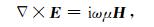
To apply finite difference methods to MT numerical modeling, one can solve the electric and magnetic fields simultaneously using

|
(1) |
|
(2) |
where μ is the air magnetic permeability, ω is the angular frequency, σ is the conductivity (the inverse of resistivity, ρ), E is the electric field, and H is the magnetic field, the time dependence for E and H is e-iωt.
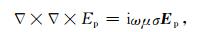
In complex domain (2-D or 3-D), to solve (1) and (2) directly requires forming a large system matrix which is time and memory consuming. In most cases, the Maxwell's equations of second order are used to solve Ep and Hp (called primary fields);
|
(3) |

|
(4) |
Then the auxiliary fields Ha and Ea are solved by (1) and (2), respectively.
There are several factors that lead to errors of the finite difference numerical solution in MT modeling [23]. Siripunvaraporn et al (2002) [8] indicated that the solutions obtained from formulas in terms of the electric fields are less sensitive to grid resolution than those obtained from the magnetic formulas. deGroot-Hedlin (2006) [24] emphasized the importance of methods used to get the auxiliary field at the surface. As 3-D MT modeling becomes popular, more and more attentions are paid to the methods used to solve linear equations; a good preconditioner together with a stable iterative solver can make the MT modeling more feasible. Han et al (2009) [25] presents a detailed comparison of 3-D MT modeling algorithms. How to find a better approximation to Maxwell's equations and a faster linear solver is an important challenge to current MT modeling studies [26].
In this paper, we make comparisons of MT finite difference numerical solutions with the analytical solutions focused on the grid resolution, ways to form system matrix and boundary conditions, aiming at what are the major factors affecting the accuracy of MT finite difference numerical solutions. We also compare the efficiency of different preconditioners combining with the linear solvers in 2-D MT cases.
2 Grid ResolutionThe errors caused by the grid resolution is nonphysical but is inherent numerical problem in finite difference methods [24]. A simple 1-D model can be used to show how grid resolution affects MT numerical solutions. In a 1-D case, the MT fields to be solved can be at the top of each layer of the homogenous layered model, denoted as H0, E0, H1, E1, …, Hn, En in Fig. 1a. We call this mode the normal grid method. When the fields to be solved are in an alternating order as H0, E1/2, …, Hn-1, En-1/2, Hn or E0, H1/2, …, En-1, Hn-1/2, En in Fig. 1a, It is called the staggered grid method [1, 5, 16, 27]. If the results of 1-D forward modeling are used to prepare boundary values for the electric polarization mode of a 2-D or 3-D model, the layers have to be extended upward to the air as the 2-D or 3-D model does.

|
Fig. 1 Relative errors of 1-D magnetotelluric fields solved by different methods of half space models in different grid resolutions. (a) A homogenous layered model with different discrete modes; (b) A 1 Ωm half space model divided with different grids respectively (Md-1 has four layers in total, the thickness of first layer is 1.6 m close to the skin depth at frequency 105 Hz; Md-2 is formed by splitting the first layer of Md-1 into two equal layers, so the first layer of Md-2 is 0.8 m; Md-3 is formed by splitting each layer of Md-1 into tow equal layers.); (c) Relative errors of electric and magnetic fields of Md-1. RE _ | Ex |; relative error of | Ex | at earth surface under Ex-Hy mode. RE_ | Hy |; relative error of | Hy | at earth surface under Ex-Hy mode. RE_ | Hy |; relative error of | Hy | at earth surface under Ex-Hy mode. RE_ | Ex |; relative error of | Ex | at the top of second layer under Ex-Hy mode. The diamonds show solutions with normal grid method, the upward triangles show solutions with staggered grid method; (d) Relative errors of electric and magnetic fields ofMd-2; (e) Relative errors of electric and magnetic fields of Md-3 |
deGroot-Hedlin et al. (1990) [28] pointed out that the spacing of the first layer should be approximately one-third of the skin depth (δ≈500 
In Fig. 1b, the homogeneous half space model of 1 Ωm is divided with different grids as Md-1, Md-2 and Md-3. The numerical solutions are obtained with the normal grid method and staggered grid method at a frequency range from 105~10-5Hz. Then we compare the MT fields by the numerical modeling with the analytical solutions. Fig. 1 (c, d, e) show the relative errors of the MT fields solved by different methods for the three half space models in Fig. 1b. The fields Ex, Hy, and Ey are at the earth's surface, that is, the top of the first layer, while the filed Hx is at the top of the second layer because the top boundary in the Hx-Ey mode is at the earth's surface and Hx at the top of the first layer is constant. In the Hx-Ey mode, the relative error of the primary field Ex (as RE_ | Hx |) of Md-2 has little improvement compared with that of Md-1, the RE_ | Hx | of Md-3 has obvious improvement compared with that of Md-2. The relative errors of the auxiliary field Hy (as RE_ | Ey |) of Md-2 and Md-3 are similar and reduced greatly compared with that of Md-1. In the Ex-Ey mode, the primary field is Ex, the RE _ | Ex | is improved steadily from Md-1 to Md-2 and Md-3, while the RE_ | Ey | has little improvement from Md-1 to Md-2, but is improved much from Md-2 to Md-3. From the images of RE-| Ey |, it seems that the staggered grid method can produce a more accurate auxiliary field in the Ex-Ey mode. In sum, by only decreasing the thickness of the first layer of the model, we can only increase the accuracy of the auxiliary field in the Hx-Ey mode and primary field in the Ex-Ey mode; but if we decrease the thickness of the first layer and keep the difference between successive rows in a reasonable range (2 times around in Md-3) simultaneously, the accuracy of both the primary field and auxiliary fields will be increased.
3 Ways to Form System MatrixWhen we use the five point difference equation to solve the second order Maxwell's equation in a 2-D case, we can define the fields in normal grids or staggered grids, the former can be divided into the normal-node method (Fig. 2a) and normal-center method (Fig. 2b). In the latter case, the fields are defined in an alternating order as Fig. 2c, we call it the staggered grid method.

|
Fig. 2 Comparison of 2-D apparent resistivity curves of two different models with normal grid and staggered grid methods, (a) The primary and auxiliary fields are defined at the same nodes of the retangular blocks, called as normal-node method; (b) The primary and auxiliary fields are defined at the center of the blocks' top edges, called as norma-center method; (c) The primary fields are defined at the center of blocks, while the auxiliary fields are defined along the blocks' edges, called as staggered grids. (d) The apparent resistivity curves of Md-4. Solid line shows analytic solution (obtained according to Refs. [11, 12]), diamonds show solutions with normal-center method, crosses show solutions with normal-node method, the upward triangles show solutions with staggered grids. (e) The apparent resistivity curves of Md-5. |
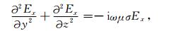
In a 2-D case, it requires some special treat-ment of the model/ is resistivity at grid nodes to obtain accurate MT solutions. From the differential form of the second order Maxwells equation in the 2-D TE mode as (5), we need to know the conductivity (σ, the inverse of resistivity ρ) at the points of the defined primary fields. The diferential form of the TM mode as (6) is a little complex; we need to know the derivatives of resistivity along both directions (y and z in Fig. 2) of the model, and the resistivity at the points of the defined primary fields.
|
(5) |
|
(6) |
The problem arises when we use the normal-center method solving equation (6). It can produce accurate solutions if the models are homogenous or homogenous in layers, but the numerical solutions deviate much from the accurate solutions when the resistivity is discontinuous laterally. We have a comparison of the numerical solutions in two cases on two 2-D models, which are Md-4 (a 2-D model with a 0. 2 km wide low resistivity abnormal zone (10 Ωm) in a 1000 Ωm haff space) and Md-5 (a 2D model with a 0.2 km wide high resistivity abnormal zone (1000 Ωm) in a 10 Ωm half space) as shown in Fig. 2 (d, e), both of which are discretized with the 47X36 mesh. In the TE mode, the apparent resistivity curves from the three methods coincide well with the analytic solutions for both Md-4 and Md-5. In the TM mode, the apparent resistivity curves of the normal-node method and staggeredgrid method coincide well with the analytic solutions, while the responses of the normalcenter method above the abnormal zone deviate more from the analytic solutions. The significantly different resistivity deviation can be found between response above the low resistivity abnormal zone in the model Md-4 at 103 Hz and response above the high resistivity abnormal zone in the model Md-5 at 10-2Hz.
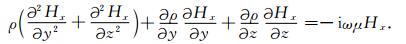
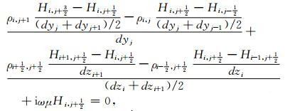
The main difficulty in the normal-center method to solve equation (6) is how to estimate the resistivity at the solution points and the difference of model’s resistivity along the horizontal direction. Although we interpolate the resistivity along y(ρy, horizontal resistivity) and z(ρz, vertical resistivity) respectively for anisotropic model at solution points, t is hard to obtain the accurate difference values of the resistivity as the solution points along the horizontal direction spanning the resistivity boundaries. The accurate responses in the TM mode with the normal-center method can be finally obtained if we use the difference form of equations (1) and (2) at the beginning and form the second order difference equation;
|
(7) |
where ρ is the model’ is resistivity at the point defined by ts subscripts, dy is the grid spacing along the horizontal direction, and dz is the grid spacing along the vertical direction. In equation (7), the resistivity at nodes are formed as;

|
(8) |
Fig. 3 shows the apparent resistivity curves obtained with equation (7) in the TM mode in comparison with the analytic solutions. It indicates that the curves above the high resistivity abnormity coincide well with the analytic solutions.

|
Fig. 3 Comparison of 2-D TM apparent resistivity curves of normal-center method with the difference equation as (7) and the analytic method. (a) The apparent resistivity curves of Md-4 at frequency 103 Hz. Solid line shows analytic solution, diamonds show solutions with normal-center method; (b) The apparent resistivity curves of Md-4 at frequency 10 -2 Hz. (c) The apparent resistivity curves of Md-5 at frequency 103 Hz. (d) The apparent resistivity curves of Md-5 at frequency 10 -2 Hz |
We construct another complex 2-D model as Md-6 m Fig. 4 to have a further test of the normal-center method, the apparent resistivity and phase curves in both TE and TM modes are obtained, and we also calculate the responses with the forward subroutine of NLCG[17]. From the results of three frequencies (as f=104 Hz, 1 Hz, 10-4 Hz) in Fig. 4, the responses of the normal-center method coincide well with the responses of the forward subroutine of NLCG except minor deviation of phase (φ) above the low resistivity abnormities at very high frequency as 104 Hz.

|
Fig. 4 Comparison of 2-D apparent resistivity and phase curves of normal-center method with the forward results of NLCG [17]. The mesh size of Md-6 is 46 × 45, only core parts of shallow level are shown here. Solid lines show the responses of Md-6 with the forward subroutine of NLCG, empty circles show solutions with normal-center method |
For the MT problem, if the Dirichlet boundary condition at the top of the model and a homogenous half space at the bottom are used, the boundary values at the lateral sides are needed to be solved in 2-D or 3-D cases. To see how much the ateral boundary values affect the solutions, we make a simple test with a 1000 Ωm half space model. We obtain the electric fields with the 1-D numerical and analytic methods at the earth surface from frequency 105~10-5 Hz firstly, and then calculate the 2-D numerical electric fields of the TE mode with the boundary values provided by 1-D numerical solution and analytic solution, respectively. Fig. 5 shows the comparison of the primary fields (including real and imaginary parts) at the earth' s surface of both 1-D and 2-D results. Though the imaginary part of the boundary 1-D values change to some extent, the primary fields of the 2-D TE mode coincide well. It means that there is limitation to increase the accuracy of the 2-D MT finite difference numerical solution only by increasing the accuracy of the boundary values. In MT finite difference numerical modeling, the main difficulties and errors are not due to the approximations made in the boundary conditions[6].

|
Fig. 5 Comparison of real and imaginary electric fields of both 1-D and 2-D solutions for a 1000 Ωm half space. Solid lines denote 1-D analytic solutions at surface; Diamonds show 1-D numerical solutions at surface; Upward triangles show 2-D numerical solutions under TE mode at surface using 1-D analytic solution as the boundary values at lateral sides; Crosses show 2-D numerical solutions under TE mode at surface using 1-D numerical solution as the boundary values at lateral sides |
If Maxwells equations are approx imated with the finite difference method in MT modeling, a linear equations Ax=b are constructed, here x is the vector made up of N unknown primary fields, and A is the system matrix with the leading dimension N. In 2-D or 3-D cases, the number N becomes very large, and the solutions of the equations are usually obtained with the preconditioned herative methods in order to avoid solving the reverse of A directly. Commonly, a preconditioner is a matrix M approximating the system matrix A to form anew system M-1 Ax=M-1b, and the new matrix M-1 A maybe more favorable to convergence.
The preconditioned Krylov subspace methods[29] are mostly used in solving MT problems. A good preconditioner is an art when it combines well with the iterative solver[30], which is very essential in 3D MT finite difference forward modeling. For example, Mackie et al. (1994)[6] used incomplete Cholesky decomposition as preconditioner for Minimum Residual (MR) algorithm and Biconju-gate Gradient (BiCG). Smith (1996)[10] found that the incomplete Cholesky preconditioner can accelerate convergence of BICG iterative method. Siripunvaraporn et al. (2002)[8] combined incomplete LU decomposition with the Quasi-Minimal Residual (QMR) method. We make a comparison of the validity of four iterative methods BiCG, QMR, Conjugate Gradient Squared (CGS), and Biconjugate Gradient Stabilized (BiCGSTAB) using a 2-D model as same as Md-4 with a 47 X 36 mesh, the desired residual is 10 -12. A Jacobi precondi-tioner (M is a diagonal matrix, its elements are the diagonal of matrix A.) is used for the four linear solvers, the convergence of both Jacobi-BICGSTAB and Jacobi-CGS are not improved at low frequencies, while Jacobi-BICG and Jacobi-QMR can reach the desired residual. Fig. 6 shows the convergence and consuming time of Jacobi-BICG and Jacobi-QMR in the TE and TM modes at frequency 1 Hz. Though the Jacobi-QMR shows a more smooth convergence than Jacobi-BICG, the former consumes more time per iteration than the latter.

|
Fig. 6 Comparison of the convergence (left) and time (right) of Jacobi-BICG and Jacobi-QMR on a 47×36 2-D MT mesh at frequency 1 Hz. Additional 15 air layers for TE mode |
The incomplete LU factorization is widely used in constructing preconditioner for the nonsymmetric system matrix, e. g. the DILU is one of the simplest incomplete LU factorization[29]. By using the DILU preconditioner, we make a further comparison of the solvers BICG, CGS, BICGSTAB and QMR on the same 2-D model Md-4 in the TE and TM modes at frequency 1 Hz. As shown in Fig. 7, all the four solvers can reach the desired residual, and the DILU-BICGSTAB takes the least iterations to reach the desired residual. Taking the example of BICG solver, the iterative number of DILU BICG decreases notably to less than one-tenth of that of Jacobi-BICG, and the total consuming time is about one-fifth of that of Jacobi-BICG. Of course, the inconsistent decrease of iterative number and the corresponding consu-ming time implies that it takes more time to construct and apply DILU preconditioner than Jacobi preconditioner.

|
Fig. 7 Comparison of the convergence (left) and time (right) of BICG, CGS, BICGSTAB, and QMR with a DILU preconditioner on a 47×36 2-D MT mesh at frequency 1 Hz. Additional 15 air layers for TE mode |
The finite difference MT numerical modeling is quickly developed, but enhancement of the accuracy of solutions is still an important task. It is necessary to study the ways to find the resistivity at nodes and their difference values, and the ways to form the system equations with an appropriate mode, for example, to divide the model with normal grids or staggered grids. Unlike the usual method to solve E first in the 2-D TE mode, Weaver et al. (1996)[13] calculated E at surface from the H solutions obtained on both types of grid. If the higher accuracy of primary fields is reached, the accuracy of auxiliary fields at the surface can also be obtained with a suitable method as that of Smith (1996)[9]. In our example of solving 2-D TM fields with the normal-center method, the difference form of the first order Maxwell’s equations (1) and (2) is used to form the secondorder difference equation (7), in which themodels’ resistivity variance and the resistivity at nodes are carefully considered and accuracy of solutions is improved.
The convergence of four solvers BICG, CGS, BICGSTAB and QMR with a Jacobi preconditioner and DILU preconditioner is discussed respectively, and it is found that the linear solvers (Jacobi-CGS and Jacobi-BICGSTAB) become stagnant at low frequencies in the 2-D case. All the four solvers BICG, CGS, BICGSTAB and QMR with DILU preconditioner can reach the desired residual in the 2-D case at frequency 1 Hz, and the efficiency of DILU preconditioner is super over Jacobi precondi-toner. Of course, DILU is one of the simplest incomplete factorization methods, and some more suitable and effective preconditioners should be tested and adopted in future research.
AcknowledgementsThis study has been supported by the Director Foundation of Institute of Geology, China Earthquake Administration (Grant No. DF-IGCEA-0608-2-16) and the National Natural Science Foundation of China (Grant No. 40534023 and Grant No. 40974042). Mr. Rodi and Mackie are acknowledged for providing their MT inversion codes NLCG. Mr. Weaver, Le Quang and Fischer are acknowledged for providing their codes to calculate 2-D analytic solutions. We also thank the anonymous reviewers and editors for their comments that lead to improvements in this paper.
| [1] | Yee K S. Numerical solution of initial boundary value problems involving Maxwell's equations in isotropic media. IEEE Trans.Ant.Prop, 1966, AP-14: 302-307. |
| [2] | Alumbaugh D L, Newman G A, Prevost L, et al. Three-dimensional wideband electromagnetic modelling on massively parallel computers. Radio Science, 1996, 31(1): 1-23. DOI:10.1029/95RS02815 |
| [3] | Aprea C, Booker J R, Smith J T. The forward problem of electromagnetic induction:accurate finite-difference approxi-mations for two-dimensional discrete boundaries with arbitrary geometry. Geophys.J.Int., 1997, 129: 29-40. DOI:10.1111/gji.1997.129.issue-1 |
| [4] | Brewitt-Taylor C R, Weaver J T. On the finite difference solution of two-dimensional induction problems. Geophys.J.Int., 1976, 47(2): 375-396. DOI:10.1111/j.1365-246X.1976.tb01280.x |
| [5] | Mackie R L, Madden T R, Wannamaker P E. Three-dimensional magnetotelluric modelling using difference equations-theory and comparison to integral equation solutions. Geophysics, 1993, 58: 215-226. DOI:10.1190/1.1443407 |
| [6] | Mackie R L, Smith J T, Madden T R. Three-dimensional magnetotelluric modelling using difference equations:The magnetotelluric example. Radio Science, 1994, 29(4): 923-935. DOI:10.1029/94RS00326 |
| [7] | Pek J, Verner T. Finite-difference modelling of magnetotelluric fields in two-dimensional anisotropic media. Geophys.J.Int., 1997, 128: 505-521. DOI:10.1111/gji.1997.128.issue-3 |
| [8] | Siripunvaraporn W, Egbert G, Lenbury Y. Numerical accuracy of magnetotelluric modelling:a comparison of finite difference approximation. Earth Planets Space, 2002, 54: 721-725. DOI:10.1186/BF03351724 |
| [9] | Smith J T. Conservative modelling of 3-D electromagnetic fields, Part I, Properties and error analysis. Geophysics, 1996, 61: 1308-1318. DOI:10.1190/1.1444054 |
| [10] | Smith J T. Conservative modelling of 3-D electromagnetic fields, Part II, Biconjugate gradient solution and an accelertor. Geophysics, 1996, 61: 1319-1324. DOI:10.1190/1.1444055 |
| [11] | Weaver J T, Le Quang B V, Fischer G. A comparison of analytic and numerical results for a two-dimensional control model in electromagnetic induction-I. B-polarization calculations.Geophys.J.Int., 1985, 82(2): 263-277. DOI:10.1111/j.1365-246X.1985.tb05137.x |
| [12] | Weaver J T, Le Quang B V, Fischer G. A comparison of analytical and numerical results for a 2-D control model in electromagnetic induction-II. E-polarization calculations.Geophys.J.Int., 1986, 87(3): 917-948. DOI:10.1111/j.1365-246X.1986.tb01977.x |
| [13] | Weaver J T, Pu X H, Agarwal A K. Improved methods for solving for the magnetic field in E-polarization induction problems with fixed and staggered grids. Geophys.J.Int., 1996, 126(2): 437-446. DOI:10.1111/gji.1996.126.issue-2 |
| [14] | Xiong Z. Domain decomposition for 3D electromagnetic modelling. Earth Planets Space, 1999, 51: 1013-1018. DOI:10.1186/BF03351574 |
| [15] | Xiong Z, Raiche A, Sugeng F. Efficient solution of full domain 3D electromagnetic modelling problems. Explor.Geophys., 2000, 31: 158-161. DOI:10.1071/EG00158 |
| [16] | Tan H D, Yu Q F, Booker J, et al. Magnetotelluric 3-D modeling using the staggered-grid finite difference method. Chinese J.Geophys.(in Chinese), 2003, 46(5): 705-711. |
| [17] | Rodi W, Mackie R L. Nonlinear conjugate gradients algorithm for 2-D magnetotelluric inversion. Geophysics, 2001, 66(1): 174-187. DOI:10.1190/1.1444893 |
| [18] | Siripunvaraporn W, Egbert G. An efficient data-subspace inversion method for 2-D magnetotelluric data. Geophysics, 2000, 65(3): 791-803. DOI:10.1190/1.1444778 |
| [19] | Smith J T, Booker J R. Rapid inversion of two-and three-dimensional magnetotelluric data. J.Geophys.Res., 1991, 96: 3905-3922. DOI:10.1029/90JB02416 |
| [20] | Mackie R L, Madden T R. Three-dimensional magnetotell-uric inversion using conjugate gradients. Geophys.J.Int., 1993, 115: 215-229. DOI:10.1111/gji.1993.115.issue-1 |
| [21] | Newman G A, Alumbaugh D L. Three dimensional mag-netotelluric inversion using non-linear conjugate gradients. Geophys.J.Int., 2000, 140: 410-424. DOI:10.1046/j.1365-246x.2000.00007.x |
| [22] | Siripunvaraporn W, Egbert G, Lenbury Y, et al. Three-dimensional magnetotelluric inversion. Data Space Method, Phys.Earth.Planet.Int., 2005, 150: 3-14. DOI:10.1016/j.pepi.2004.08.023 |
| [23] | Zhdanov M S, Varentsov I M, Weaver J T, et al. Methods for modelling electromagnetic fields results from COMMEMI-The international project on the comparison of modelling methods for electromagnetic induction. Journal of Applied Geophysics, 1997, 37: 133-271. DOI:10.1016/S0926-9851(97)00013-X |
| [24] | deGroot-Hedlin C. Finite-difference modelling of mag-netotelluric fields:error estimates for uniform and nonuniform grids. Geophysics, 2006, 71(3): 97-106. DOI:10.1190/1.2195991 |
| [25] | Han N, Nam M J, Kim H J, et al. A comparison of accuracy and computation time of three-dimensional magnetotelluric modelling algorithms. J.Geophys.Eng., 2009, 6: 136-145. DOI:10.1088/1742-2132/6/2/005 |
| [26] | Avdeev D B. Three-dimensional electromagnetic modelling and inversion from theory to application. Surveys in Geophysics, 2005, 26: 767-799. DOI:10.1007/s10712-005-1836-x |
| [27] | Li Z H, Huang Q H, Wang Y B. A 3-D staggered grid PSTD method for borehole radar simulations in dispersive media. Chinese J.Geophys.(in Chinese), 2009, 52(7): 1915-1922. |
| [28] | deGroot-Hedlin C, Constable S. Occam inversion to create smooth 2-dimensional models from magnetotelluric data. Geophysics, 1990, 55: 1613-1624. DOI:10.1190/1.1442813 |
| [29] | Barrett R, Berry M, Chan T, et al. Templates for the Solution of Linear Systems:Building Blocks for Iterative Methods. SIAM, 1994. |
| [30] | Saad Y. Iterative Methods for Sparse Linear Systems. (Second Edition). Philadelphia: SIAM, 2000. |